Timescaledb - Tutorials

Pages: 12

Advanced data management

URL: llms-txt#advanced-data-management

Contents:

Hypertable chunk time intervals and automation policies
Automatically delete older tick data
Automatically delete older candlestick data
Automatically compress tick data
Automatically compress candlestick data

The final part of this tutorial shows you some more advanced techniques to efficiently manage your tick and candlestick data long-term. TimescaleDB is equipped with multiple features that help you manage your data lifecycle and reduce your disk storage needs as your data grows.

This section contains four examples of how you can set up automation policies on your tick data hypertable and your candlestick continuous aggregates. This can help you save on disk storage and improve the performance of long-range analytical queries by automatically:

Deleting older tick data
Deleting older candlestick data
Compressing tick data
Compressing candlestick data

Before you implement any of these automation policies, it's important to have a high-level understanding of chunk time intervals in TimescaleDB hypertables and continuous aggregates. The chunk time interval you set for your tick data table directly affects how these automation policies work. For more information, see the [hypertables and chunks][chunks] section.

Hypertable chunk time intervals and automation policies

TimescaleDB uses hypertables to provide a high-level and familiar abstraction layer to interact with Postgres tables. You just need to access one hypertable to access all of your time-series data.

Under the hood, TimescaleDB creates chunks based on the timestamp column. Each chunk size is determined by the [chunk_time_interval][interval] parameter. You can provide this parameter when creating the hypertable, or you can change it afterwards. If you don't provide this optional parameter, the chunk time interval defaults to 7 days. This means that each of the chunks in the hypertable contains 7 days' worth of data.

Knowing your chunk time interval is important. All of the TimescaleDB automation policies described in this section depend on this information, and the chunk time interval fundamentally affects how these policies impact your data.

In this section, learn about these automation policies and how they work in the context of financial tick data.

Automatically delete older tick data

Usually, the older your time-series data, the less relevant and useful it is. This is often the case with tick data as well. As time passes, you might not need the raw tick data any more, because you only want to query the candlestick aggregations. In this scenario, you can decide to remove tick data automatically from your hypertable after it gets older than a certain time interval.

TimescaleDB has a built-in way to automatically remove raw data after a specific time. You can set up this automation using a [data retention policy][retention]:

When you run this, it adds a data retention policy to the crypto_ticks hypertable that removes a chunk after all the data in the chunk becomes older than 7 days. All records in the chunk need to be older than 7 days before the chunk is dropped.

Knowledge of your hypertable's chunk time interval is crucial here. If you were to set a data retention policy with INTERVAL '3 days', the policy would not remove any data after three days, because your chunk time interval is seven days. Even after three days have passed, the most recent chunk still contains data that is newer than three days, and so cannot be removed by the data retention policy.

If you want to change this behavior, and drop chunks more often and sooner, experiment with different chunk time intervals. For example, if you set the chunk time interval to be two days only, you could create a retention policy with a 2-day interval that would drop a chunk every other day (assuming you're ingesting data in the meantime).

For more information, see the [data retention][retention] section.

Make sure none of the continuous aggregate policies intersect with a data retention policy. It's possible to keep the candlestick data in the continuous aggregate and drop tick data from the underlying hypertable, but only if you materialize data in the continuous aggregate first, before the data is dropped from the underlying hypertable.

Automatically delete older candlestick data

Deleting older raw tick data from your hypertable while retaining aggregate views for longer periods is a common way of minimizing disk utilization. However, deleting older candlestick data from the continuous aggregates can provide another method for further control over long-term disk use. TimescaleDB allows you to create data retention policies on continuous aggregates as well.

Continuous aggregates also have chunk time intervals because they use hypertables in the background. By default, the continuous aggregate's chunk time interval is 10 times what the original hypertable's chunk time interval is. For example, if the original hypertable's chunk time interval is 7 days, the continuous aggregates that are on top of it will have a 70 day chunk time interval.

You can set up a data retention policy to remove old data from your one_min_candle continuous aggregate:

This data retention policy removes chunks from the continuous aggregate that are older than 70 days. In TimescaleDB, this is determined by the range_end property of a hypertable, or in the case of a continuous aggregate, the materialized hypertable. In practice, this means that if you were to define a data retention policy of 30 days for a continuous aggregate that has a chunk_time_interval of 70 days, data would not be removed from the continuous aggregates until the range_end of a chunk is at least 70 days older than the current time, due to the chunk time interval of the original hypertable.

Automatically compress tick data

TimescaleDB allows you to keep your tick data in the hypertable but still save on storage costs with TimescaleDB's native compression. You need to enable compression on the hypertable and set up a compression policy to automatically compress old data.

Enable compression on crypto_ticks hypertable:

Set up compression policy to compress data that's older than 7 days:

Executing these two SQL scripts compresses chunks that are older than 7 days.

For more information, see the [compression][compression] section.

Automatically compress candlestick data

Beginning with [TimescaleDB 2.6][release-blog], you can also set up a compression policy on your continuous aggregates. This is a useful feature if you store a lot of historical candlestick data that consumes significant disk space, but you still want to retain it for longer periods.

Enable compression on the one_min_candle view:

Add a compression policy to compress data after 70 days:

Before setting a compression policy on any of the candlestick views, set a refresh policy first. The compression policy interval should be set so that actively refreshed time intervals are not compressed.

[Read more about compressing continuous aggregates.][caggs-compress]

===== PAGE: https://docs.tigerdata.com/tutorials/energy-data/dataset-energy/ =====

Examples:

Example 1 (sql):

SELECT add_retention_policy('crypto_ticks', INTERVAL '7 days');

Example 2 (sql):

SELECT add_retention_policy('one_min_candle', INTERVAL '70 days');

Example 3 (sql):

ALTER TABLE crypto_ticks SET (
 timescaledb.compress,
 timescaledb.compress_segmentby = 'symbol'
);

Example 4 (sql):

SELECT add_compression_policy('crypto_ticks', INTERVAL '7 days');

Tutorials

URL: llms-txt#tutorials

Tiger Data tutorials are designed to help you get up and running with Tiger Data products. They walk you through a variety of scenarios using example datasets, to teach you how to construct interesting queries, find out what information your database has hidden in it, and even give you options for visualizing and graphing your results.

Real-time analytics
- [Analytics on energy consumption][rta-energy]: make data-driven decisions using energy consumption data.
- [Analytics on transport and geospatial data][rta-transport]: optimize profits using geospatial transport data.
Cryptocurrency
- [Query the Bitcoin blockchain][beginner-crypto]: do your own research on the Bitcoin blockchain.
- [Analyze the Bitcoin blockchain][intermediate-crypto]: discover the relationship between transactions, blocks, fees, and miner revenue.
Finance
- [Analyze financial tick data][beginner-finance]: chart the trading highs and lows for your favorite stock.
- [Ingest real-time financial data using WebSocket][advanced-finance]: use a websocket connection to visualize the trading highs and lows for your favorite stock.
IoT
- [Simulate an IoT sensor dataset][iot]: simulate an IoT sensor dataset and run simple queries on it.
Cookbooks
- [Tiger community cookbook][cookbooks]: get suggestions from the Tiger community about how to resolve common issues.

===== PAGE: https://docs.tigerdata.com/_troubleshooting/compression-dml-tuple-limit/ =====

Query time-series data tutorial - set up dataset

URL: llms-txt#query-time-series-data-tutorial---set-up-dataset

Contents:

Prerequisites
Optimize time-series data in hypertables
Create standard Postgres tables for relational data
Load trip data

This tutorial uses a dataset that contains historical data from the New York City Taxi and Limousine Commission [NYC TLC][nyc-tlc], in a hypertable named rides. It also includes a separate tables of payment types and rates, in a regular Postgres table named payment_types, and rates.

To follow the steps on this page:

Create a target [Tiger Cloud service][create-service] with the Real-time analytics capability.

You need [your connection details][connection-info]. This procedure also works for [self-hosted TimescaleDB][enable-timescaledb].

Optimize time-series data in hypertables

Time-series data represents how a system, process, or behavior changes over time. [Hypertables][hypertables-section] are Postgres tables that help you improve insert and query performance by automatically partitioning your data by time. Each hypertable is made up of child tables called chunks. Each chunk is assigned a range of time, and only contains data from that range.

Hypertables exist alongside regular Postgres tables. You interact with hypertables and regular Postgres tables in the same way. You use regular Postgres tables for relational data.

Create a hypertable to store the taxi trip data

If you are self-hosting TimescaleDB v2.19.3 and below, create a [Postgres relational table][pg-create-table], then convert it using [create_hypertable][create_hypertable]. You then enable hypercore with a call to [ALTER TABLE][alter_table_hypercore].

Add another dimension to partition your hypertable more efficiently
Create an index to support efficient queries

Index by vendor, rate code, and passenger count:

Create standard Postgres tables for relational data

When you have other relational data that enhances your time-series data, you can create standard Postgres tables just as you would normally. For this dataset, there are two other tables of data, called payment_types and rates.

Add a relational table to store the payment types data
Add a relational table to store the rates data

You can confirm that the scripts were successful by running the \dt command in the psql command line. You should see this:

When you have your database set up, you can load the taxi trip data into the rides hypertable.

This is a large dataset, so it might take a long time, depending on your network connection.

Download the dataset:

nyc_data.tar.gz

Use your file manager to decompress the downloaded dataset, and take a note of the path to the nyc_data_rides.csv file.
At the psql prompt, copy the data from the nyc_data_rides.csv file into your hypertable. Make sure you point to the correct path, if it is not in your current working directory:

You can check that the data has been copied successfully with this command:

You should get five records that look like this:

===== PAGE: https://docs.tigerdata.com/tutorials/nyc-taxi-cab/index/ =====

Examples:

Example 1 (sql):

CREATE TABLE "rides"(
        vendor_id TEXT,
        pickup_datetime TIMESTAMP WITHOUT TIME ZONE NOT NULL,
        dropoff_datetime TIMESTAMP WITHOUT TIME ZONE NOT NULL,
        passenger_count NUMERIC,
        trip_distance NUMERIC,
        pickup_longitude  NUMERIC,
        pickup_latitude   NUMERIC,
        rate_code         INTEGER,
        dropoff_longitude NUMERIC,
        dropoff_latitude  NUMERIC,
        payment_type INTEGER,
        fare_amount NUMERIC,
        extra NUMERIC,
        mta_tax NUMERIC,
        tip_amount NUMERIC,
        tolls_amount NUMERIC,
        improvement_surcharge NUMERIC,
        total_amount NUMERIC
    ) WITH (
       tsdb.hypertable,
       tsdb.partition_column='pickup_datetime',
       tsdb.create_default_indexes=false
    );

Example 2 (sql):

SELECT add_dimension('rides', by_hash('payment_type', 2));

Example 3 (sql):

CREATE INDEX ON rides (vendor_id, pickup_datetime DESC);
    CREATE INDEX ON rides (rate_code, pickup_datetime DESC);
    CREATE INDEX ON rides (passenger_count, pickup_datetime DESC);

Example 4 (sql):

CREATE TABLE IF NOT EXISTS "payment_types"(
        payment_type INTEGER,
        description TEXT
    );
    INSERT INTO payment_types(payment_type, description) VALUES
    (1, 'credit card'),
    (2, 'cash'),
    (3, 'no charge'),
    (4, 'dispute'),
    (5, 'unknown'),
    (6, 'voided trip');

Plot geospatial time-series data tutorial

URL: llms-txt#plot-geospatial-time-series-data-tutorial

Contents:

Prerequisites
Steps in this tutorial
About querying data with Timescale

New York City is home to about 9 million people. This tutorial uses historical data from New York's yellow taxi network, provided by the New York City Taxi and Limousine Commission [NYC TLC][nyc-tlc]. The NYC TLC tracks over 200,000 vehicles making about 1 million trips each day. Because nearly all of this data is time-series data, proper analysis requires a purpose-built time-series database, like Timescale.

In the [beginner NYC taxis tutorial][beginner-fleet], you looked at constructing queries that looked at how many rides were taken, and when. The NYC taxi cab dataset also contains information about where each ride was picked up. This is geospatial data, and you can use a Postgres extension called PostGIS to examine where rides are originating from. Additionally, you can visualize the data in Grafana, by overlaying it on a map.

Before you begin, make sure you have:

Signed up for a [free Tiger Data account][cloud-install].
[](#) If you want to graph your queries, signed up for a [Grafana account][grafana-setup].

Steps in this tutorial

This tutorial covers:

[Setting up your dataset][dataset-nyc]: Set up and connect to a Timescale service, and load data into your database using psql.
[Querying your dataset][query-nyc]: Analyze a dataset containing NYC taxi trip data using Tiger Cloud and Postgres, and plot the results in Grafana.

About querying data with Timescale

This tutorial uses the [NYC taxi data][nyc-tlc] to show you how to construct queries for geospatial time-series data. The analysis you do in this tutorial is similar to the kind of analysis civic organizations do to plan new roads and public services.

It starts by teaching you how to set up and connect to a Tiger Cloud service, create tables, and load data into the tables using psql. If you have already completed the [first NYC taxis tutorial][beginner-fleet], then you already have the dataset loaded, and you can skip [straight to the queries][plot-nyc].

You then learn how to conduct analysis and monitoring on your dataset. It walks you through using Postgres queries with the PostGIS extension to obtain information, and plotting the results in Grafana.

===== PAGE: https://docs.tigerdata.com/tutorials/nyc-taxi-geospatial/plot-nyc/ =====

Query candlestick views

URL: llms-txt#query-candlestick-views

Contents:

1-min BTC/USD candlestick chart
1-hour BTC/USD candlestick chart
1-day BTC/USD candlestick chart
BTC vs. ETH 1-day price changes delta line chart

So far in this tutorial, you have created the schema to store tick data, and set up multiple candlestick views. In this section, use some example candlestick queries and see how they can be represented in data visualizations.

The queries in this section are example queries. The sample data provided with this tutorial is updated on a regular basis to have near-time data, typically no more than a few days old. Our sample queries reflect time filters that might be longer than you would normally use, so feel free to modify the time filter in the WHERE clause as the data ages, or as you begin to insert updated tick readings.

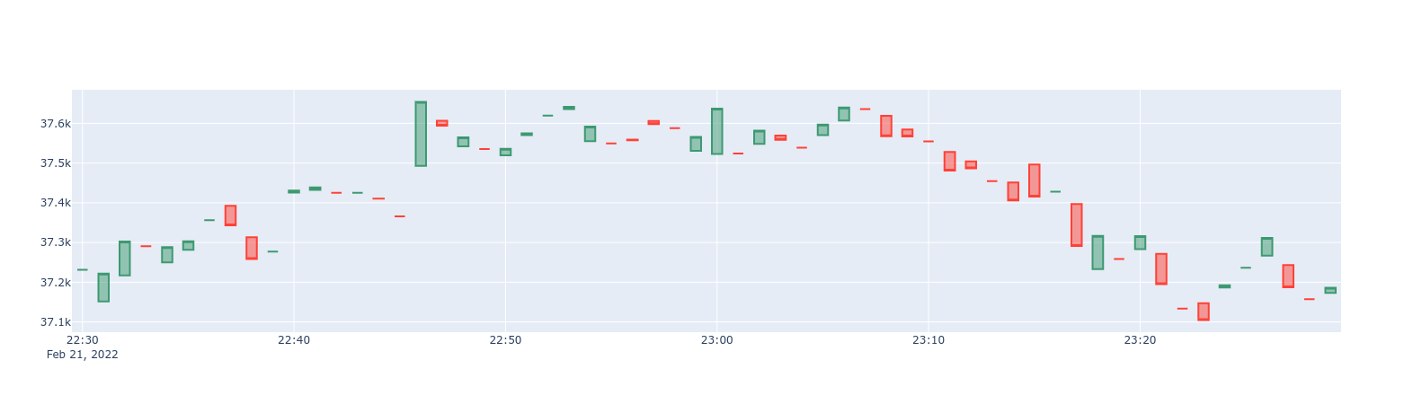
1-min BTC/USD candlestick chart

Start with a one_min_candle continuous aggregate, which contains 1-min candlesticks:

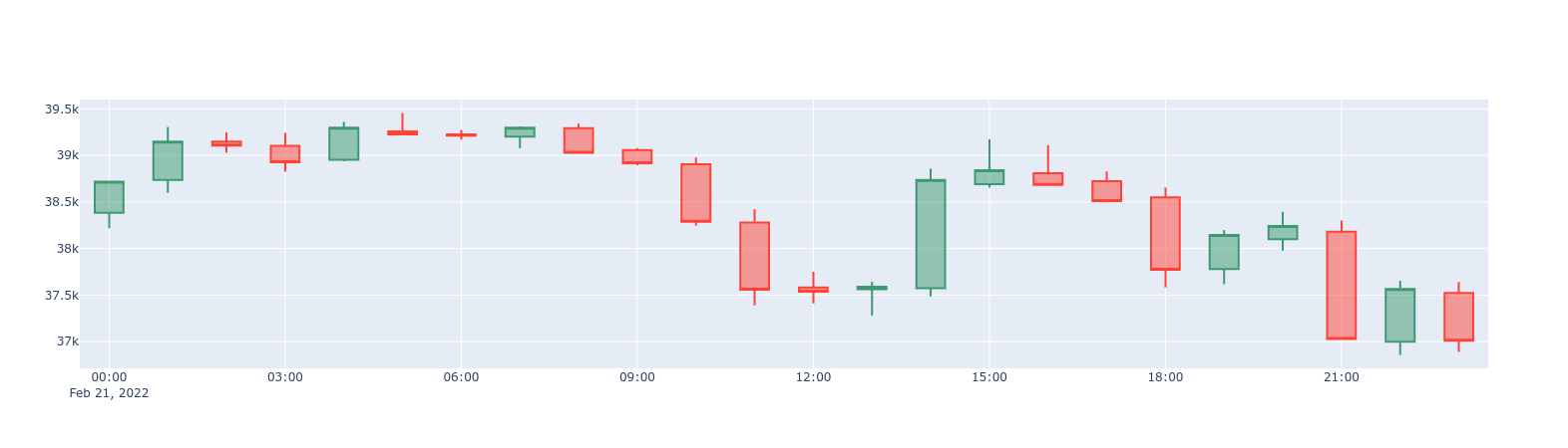
1-hour BTC/USD candlestick chart

If you find that 1-min candlesticks are too granular, you can query the one_hour_candle continuous aggregate containing 1-hour candlesticks:

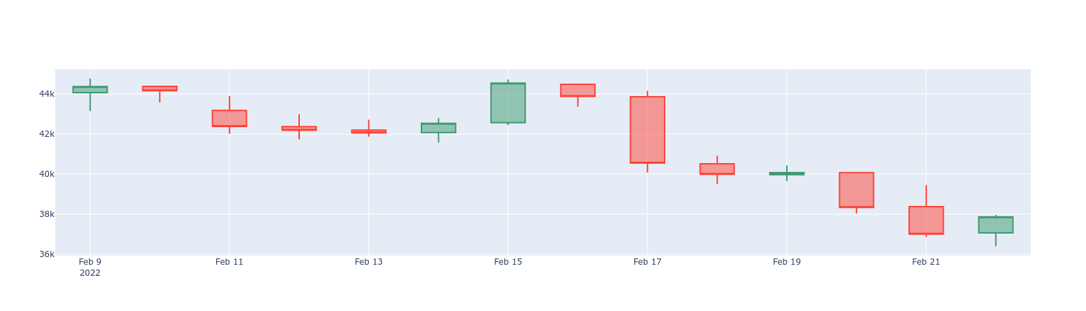
1-day BTC/USD candlestick chart

To zoom out even more, query the one_day_candle continuous aggregate, which has one-day candlesticks:

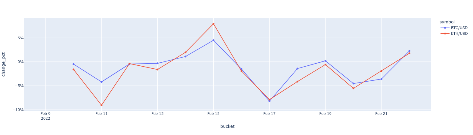
BTC vs. ETH 1-day price changes delta line chart

You can calculate and visualize the price change differences between two symbols. In a previous example, you saw how to do this by comparing the opening and closing prices. But what if you want to compare today's closing price with yesterday's closing price? Here's an example how you can achieve this by using the [LAG()][lag] window function on an already existing candlestick view:

===== PAGE: https://docs.tigerdata.com/tutorials/OLD-financial-candlestick-tick-data/design-tick-schema/ =====

Examples:

Example 1 (sql):

SELECT * FROM one_min_candle
WHERE symbol = 'BTC/USD' AND bucket >= NOW() - INTERVAL '24 hour'
ORDER BY bucket

Example 2 (sql):

SELECT * FROM one_hour_candle
WHERE symbol = 'BTC/USD' AND bucket >= NOW() - INTERVAL '2 day'
ORDER BY bucket

Example 3 (sql):

SELECT * FROM one_day_candle
WHERE symbol = 'BTC/USD' AND bucket >= NOW() - INTERVAL '14 days'
ORDER BY bucket

Example 4 (sql):

SELECT *, ("close" - LAG("close", 1) OVER (PARTITION BY symbol ORDER BY bucket)) / "close" AS change_pct
FROM one_day_candle
WHERE symbol IN ('BTC/USD', 'ETH/USD') AND bucket >= NOW() - INTERVAL '14 days'
ORDER BY bucket

Query time-series data tutorial

URL: llms-txt#query-time-series-data-tutorial

Contents:

Prerequisites
Steps in this tutorial
About querying data with Timescale

Before you begin, make sure you have:

Signed up for a [free Tiger Data account][cloud-install].

Steps in this tutorial

This tutorial covers:

[Setting up your dataset][dataset-nyc]: Set up and connect to a Timescale service, and load data into your database using psql.
[Querying your dataset][query-nyc]: Analyze a dataset containing NYC taxi trip data using Tiger Cloud and Postgres.
[Bonus: Store data efficiently][compress-nyc]: Learn how to store and query your NYC taxi trip data more efficiently using compression feature of Timescale.

About querying data with Timescale

This tutorial uses the [NYC taxi data][nyc-tlc] to show you how to construct queries for time-series data. The analysis you do in this tutorial is similar to the kind of analysis data science organizations use to do things like plan upgrades, set budgets, and allocate resources.

It starts by teaching you how to set up and connect to a Tiger Cloud service, create tables, and load data into the tables using psql.

You then learn how to conduct analysis and monitoring on your dataset. It walks you through using Postgres queries to obtain information, including how to use JOINs to combine your time-series data with relational or business data.

If you have been provided with a pre-loaded dataset on your Tiger Cloud service, go directly to the queries section.

===== PAGE: https://docs.tigerdata.com/tutorials/nyc-taxi-cab/query-nyc/ =====

Energy consumption data tutorial - query the data

URL: llms-txt#energy-consumption-data-tutorial---query-the-data

Contents:

What is the energy consumption by the hour of the day?
- Finding how many kilowatts of energy is consumed on an hourly basis
What is the energy consumption by the day of the week?
- Finding energy consumption during the weekdays
What is the energy consumption on a monthly basis?
- Finding energy consumption for each month of the year

When you have your dataset loaded, you can start constructing some queries to discover what your data tells you. This tutorial uses [TimescaleDB hyperfunctions][about-hyperfunctions] to construct queries that are not possible in standard Postgres.

In this section, you learn how to construct queries, to answer these questions:

Energy consumption by hour of day
Energy consumption by weekday.
Energy consumption by month.

What is the energy consumption by the hour of the day?

When you have your database set up for energy consumption data, you can construct a query to find the median and the maximum consumption of energy on an hourly basis in a typical day.

Finding how many kilowatts of energy is consumed on an hourly basis

Connect to the Tiger Cloud service that contains the energy consumption dataset.
At the psql prompt, use the TimescaleDB Toolkit functionality to get calculate the fiftieth percentile or the median. Then calculate the maximum energy consumed using the standard Postgres max function:
The data you get back looks a bit like this:

What is the energy consumption by the day of the week?

You can also check how energy consumption varies between weekends and weekdays.

Finding energy consumption during the weekdays

Connect to the Tiger Cloud service that contains the energy consumption dataset.
At the psql prompt, use this query to find difference in consumption during the weekdays and the weekends:
The data you get back looks a bit like this:

What is the energy consumption on a monthly basis?

You may also want to check the energy consumption that occurs on a monthly basis.

Finding energy consumption for each month of the year

Connect to the Tiger Cloud service that contains the energy consumption dataset.
At the psql prompt, use this query to find consumption for each month of the year:
The data you get back looks a bit like this:
[](#) To visualize this in Grafana, create a new panel, and select the Bar Chart visualization. Select the energy consumption dataset as your data source, and type the query from the previous step. In the Format as section, select Table.
[](#) Select a color scheme so that different consumptions are shown in different colors. In the options panel, under Standard options, change the Color scheme to a useful by value range.

<img

class="main-content__illustration"
src="https://assets.timescale.com/docs/images/grafana-energy.webp"
width={1375} height={944}
alt="Visualizing energy consumptions in Grafana"
/>

===== PAGE: https://docs.tigerdata.com/tutorials/energy-data/index/ =====

Examples:

Example 1 (sql):

WITH per_hour AS (
    SELECT
    time,
    value
    FROM kwh_hour_by_hour
    WHERE "time" at time zone 'Europe/Berlin' > date_trunc('month', time) - interval '1 year'
    ORDER BY 1
    ), hourly AS (
     SELECT
          extract(HOUR FROM time) * interval '1 hour' as hour,
          value
     FROM per_hour
    )
    SELECT
        hour,
        approx_percentile(0.50, percentile_agg(value)) as median,
        max(value) as maximum
    FROM hourly
    GROUP BY 1
    ORDER BY 1;

Example 2 (sql):

hour   |       median       | maximum
        ----------+--------------------+---------
         00:00:00 | 0.5998949812512439 |     0.6
         01:00:00 | 0.5998949812512439 |     0.6
         02:00:00 | 0.5998949812512439 |     0.6
         03:00:00 | 1.6015944383271534 |     1.9
         04:00:00 | 2.5986701108275327 |     2.7
         05:00:00 | 1.4007385207185301 |     3.4
         06:00:00 | 0.5998949812512439 |     2.7
         07:00:00 | 0.6997720645753496 |     0.8
         08:00:00 | 0.6997720645753496 |     0.8
         09:00:00 | 0.6997720645753496 |     0.8
         10:00:00 | 0.9003240409125329 |     1.1
         11:00:00 | 0.8001143897618259 |     0.9

Example 3 (sql):

WITH per_day AS (
     SELECT
       time,
       value
     FROM kwh_day_by_day
     WHERE "time" at time zone 'Europe/Berlin' > date_trunc('month', time) - interval '1 year'
     ORDER BY 1
    ), daily AS (
        SELECT
           to_char(time, 'Dy') as day,
           value
        FROM per_day
    ), percentile AS (
        SELECT
            day,
            approx_percentile(0.50, percentile_agg(value)) as value
        FROM daily
        GROUP BY 1
        ORDER BY 1
    )
    SELECT
        d.day,
        d.ordinal,
        pd.value
    FROM unnest(array['Sun', 'Mon', 'Tue', 'Wed', 'Thu', 'Fri', 'Sat']) WITH ORDINALITY AS d(day, ordinal)
    LEFT JOIN percentile pd ON lower(pd.day) = lower(d.day);

Example 4 (sql):

day | ordinal |       value
    -----+---------+--------------------
     Mon |       2 |  23.08078714975423
     Sun |       1 | 19.511430831944395
     Tue |       3 | 25.003118897837307
     Wed |       4 |   8.09300571759772
     Sat |       7 |
     Fri |       6 |
     Thu |       5 |

Query time-series data tutorial - query the data

URL: llms-txt#query-time-series-data-tutorial---query-the-data

Contents:

How many rides take place every day?
- Finding how many rides take place every day
What is the average fare amount?
- Finding the average fare amount
How many rides of each rate type were taken?
- Finding the number of rides for each fare type
- Displaying the number of rides for each fare type
What kind of trips are going to and from airports
- Finding what kind of trips are going to and from airports
How many rides took place on New Year's Day 2016?

When you have your dataset loaded, you can start constructing some queries to discover what your data tells you. In this section, you learn how to write queries that answer these questions:

How many rides take place each day?
What is the average fare amount?
How many rides of each rate type were taken?
What kind of trips are going to and from airports?
How many rides took place on New Year's Day 2016?

How many rides take place every day?

This dataset contains ride data for January 2016. To find out how many rides took place each day, you can use a SELECT statement. In this case, you want to count the total number of rides each day, and show them in a list by date.

Finding how many rides take place every day

Connect to the Tiger Cloud service that contains the NYC taxi dataset.
At the psql prompt, use this query to select all rides taken in the first week of January 2016, and return a count of rides for each day:

The result of the query looks like this:

What is the average fare amount?

You can include a function in your SELECT query to determine the average fare paid by each passenger.

Finding the average fare amount

Connect to the Tiger Cloud service that contains the NYC taxi dataset.
At the psql prompt, use this query to select all rides taken in the first week of January 2016, and return the average fare paid on each day:

The result of the query looks like this:

How many rides of each rate type were taken?

Taxis in New York City use a range of different rate types for different kinds of trips. For example, trips to the airport are charged at a flat rate from any location within the city. This section shows you how to construct a query that shows you the nuber of trips taken for each different fare type. It also uses a JOIN statement to present the data in a more informative way.

Finding the number of rides for each fare type

Connect to the Tiger Cloud service that contains the NYC taxi dataset.
At the psql prompt, use this query to select all rides taken in the first week of January 2016, and return the total number of trips taken for each rate code:

The result of the query looks like this:

This output is correct, but it's not very easy to read, because you probably don't know what the different rate codes mean. However, the rates table in the dataset contains a human-readable description of each code. You can use a JOIN statement in your query to connect the rides and rates tables, and present information from both in your results.

Displaying the number of rides for each fare type

Connect to the Tiger Cloud service that contains the NYC taxi dataset.
At the psql prompt, copy this query to select all rides taken in the first week of January 2016, join the rides and rates tables, and return the total number of trips taken for each rate code, with a description of the rate code:

The result of the query looks like this:

What kind of trips are going to and from airports

There are two primary airports in the dataset: John F. Kennedy airport, or JFK, is represented by rate code 2; Newark airport, or EWR, is represented by rate code 3.

Information about the trips that are going to and from the two airports is useful for city planning, as well as for organizations like the NYC Tourism Bureau.

This section shows you how to construct a query that returns trip information for trips going only to the new main airports.

Finding what kind of trips are going to and from airports

Connect to the Tiger Cloud service that contains the NYC taxi dataset.
At the psql prompt, use this query to select all rides taken to and from JFK and Newark airports, in the first week of January 2016, and return the number of trips to that airport, the average trip duration, average trip cost, and average number of passengers:

The result of the query looks like this:

How many rides took place on New Year's Day 2016?

New York City is famous for the Ball Drop New Year's Eve celebration in Times Square. Thousands of people gather to bring in the New Year and then head out into the city: to their favorite bar, to gather with friends for a meal, or back home. This section shows you how to construct a query that returns the number of taxi trips taken on 1 January, 2016, in 30 minute intervals.

In Postgres, it's not particularly easy to segment the data by 30 minute time intervals. To do this, you would need to use a TRUNC function to calculate the quotient of the minute that a ride began in divided by 30, then truncate the result to take the floor of that quotient. When you had that result, you could multiply the truncated quotient by 30.

In your Tiger Cloud service, you can use the time_bucket function to segment the data into time intervals instead.

Finding how many rides took place on New Year's Day 2016

Connect to the Tiger Cloud service that contains the NYC taxi dataset.
At the psql prompt, use this query to select all rides taken on the first day of January 2016, and return a count of rides for each 30 minute interval:

The result of the query starts like this:

===== PAGE: https://docs.tigerdata.com/tutorials/nyc-taxi-cab/compress-nyc/ =====

Examples:

Example 1 (sql):

SELECT date_trunc('day', pickup_datetime) as day,
    COUNT(*) FROM rides
    WHERE pickup_datetime < '2016-01-08'
    GROUP BY day
    ORDER BY day;

Example 2 (sql):

day         | count
    ---------------------+--------
     2016-01-01 00:00:00 | 345037
     2016-01-02 00:00:00 | 312831
     2016-01-03 00:00:00 | 302878
     2016-01-04 00:00:00 | 316171
     2016-01-05 00:00:00 | 343251
     2016-01-06 00:00:00 | 348516
     2016-01-07 00:00:00 | 364894

Example 3 (sql):

SELECT date_trunc('day', pickup_datetime)
    AS day, avg(fare_amount)
    FROM rides
    WHERE pickup_datetime < '2016-01-08'
    GROUP BY day
    ORDER BY day;

Example 4 (sql):

day         |         avg
    ---------------------+---------------------
     2016-01-01 00:00:00 | 12.8569325028909943
     2016-01-02 00:00:00 | 12.4344713599355563
     2016-01-03 00:00:00 | 13.0615900461571986
     2016-01-04 00:00:00 | 12.2072927308323660
     2016-01-05 00:00:00 | 12.0018670885154013
     2016-01-06 00:00:00 | 12.0002329017893009
     2016-01-07 00:00:00 | 12.1234180337303436

Plot geospatial time-series data tutorial - set up dataset

URL: llms-txt#plot-geospatial-time-series-data-tutorial---set-up-dataset

Contents:

Prerequisites
Optimize time-series data in hypertables
Create standard Postgres tables for relational data
Load trip data
Connect Grafana to Tiger Cloud

To follow the steps on this page:

Create a target [Tiger Cloud service][create-service] with the Real-time analytics capability.

You need [your connection details][connection-info]. This procedure also works for [self-hosted TimescaleDB][enable-timescaledb].

Optimize time-series data in hypertables

Hypertables exist alongside regular Postgres tables. You interact with hypertables and regular Postgres tables in the same way. You use regular Postgres tables for relational data.

Create a hypertable to store the taxi trip data

Add another dimension to partition your hypertable more efficiently
Create an index to support efficient queries

Index by vendor, rate code, and passenger count:

Create standard Postgres tables for relational data

Add a relational table to store the payment types data
Add a relational table to store the rates data

You can confirm that the scripts were successful by running the \dt command in the psql command line. You should see this:

When you have your database set up, you can load the taxi trip data into the rides hypertable.

This is a large dataset, so it might take a long time, depending on your network connection.

Download the dataset:

nyc_data.tar.gz

Use your file manager to decompress the downloaded dataset, and take a note of the path to the nyc_data_rides.csv file.
At the psql prompt, copy the data from the nyc_data_rides.csv file into your hypertable. Make sure you point to the correct path, if it is not in your current working directory:

You can check that the data has been copied successfully with this command:

You should get five records that look like this:

Connect Grafana to Tiger Cloud

To visualize the results of your queries, enable Grafana to read the data in your service:

Log in to Grafana

In your browser, log in to either:

- Self-hosted Grafana: at `http://localhost:3000/`. The default credentials are `admin`, `admin`.
- Grafana Cloud: use the URL and credentials you set when you created your account.

Add your service as a data source
1. Open Connections > Data sources, then click Add new data source.
2. Select PostgreSQL from the list.
3. Configure the connection:
  - Host URL, Database name, Username, and Password

Configure using your [connection details][connection-info]. Host URL is in the format <host>:<port>.

  - `TLS/SSL Mode`: select `require`.
  - `PostgreSQL options`: enable `TimescaleDB`.
  - Leave the default setting for all other fields.

Click Save & test.

Grafana checks that your details are set correctly.

===== PAGE: https://docs.tigerdata.com/tutorials/nyc-taxi-geospatial/index/ =====

Examples:

Example 1 (sql):

CREATE TABLE "rides"(
        vendor_id TEXT,
        pickup_datetime TIMESTAMP WITHOUT TIME ZONE NOT NULL,
        dropoff_datetime TIMESTAMP WITHOUT TIME ZONE NOT NULL,
        passenger_count NUMERIC,
        trip_distance NUMERIC,
        pickup_longitude  NUMERIC,
        pickup_latitude   NUMERIC,
        rate_code         INTEGER,
        dropoff_longitude NUMERIC,
        dropoff_latitude  NUMERIC,
        payment_type INTEGER,
        fare_amount NUMERIC,
        extra NUMERIC,
        mta_tax NUMERIC,
        tip_amount NUMERIC,
        tolls_amount NUMERIC,
        improvement_surcharge NUMERIC,
        total_amount NUMERIC
    ) WITH (
       tsdb.hypertable,
       tsdb.partition_column='pickup_datetime',
       tsdb.create_default_indexes=false
    );

Example 2 (sql):

SELECT add_dimension('rides', by_hash('payment_type', 2));

Example 3 (sql):

CREATE INDEX ON rides (vendor_id, pickup_datetime DESC);
    CREATE INDEX ON rides (rate_code, pickup_datetime DESC);
    CREATE INDEX ON rides (passenger_count, pickup_datetime DESC);

Example 4 (sql):

CREATE TABLE IF NOT EXISTS "payment_types"(
        payment_type INTEGER,
        description TEXT
    );
    INSERT INTO payment_types(payment_type, description) VALUES
    (1, 'credit card'),
    (2, 'cash'),
    (3, 'no charge'),
    (4, 'dispute'),
    (5, 'unknown'),
    (6, 'voided trip');

Energy consumption data tutorial

URL: llms-txt#energy-consumption-data-tutorial

Contents:

Prerequisites
Steps in this tutorial
About querying data with Timescale

When you are planning to switch to a rooftop solar system, it isn't easy, even with a specialist at hand. You need details of your power consumption, typical usage hours, distribution over a year, and other information. Collecting consumption data at the granularity of a few seconds and then getting insights on it is key - and this is what TimescaleDB is best at.

This tutorial uses energy consumption data from a typical household for over a year. You construct queries that look at how many watts were consumed, and when. Additionally, you can visualize the energy consumption data in Grafana.

Before you begin, make sure you have:

Signed up for a [free Tiger Data account][cloud-install].
[](#) [Signed up for a Grafana account][grafana-setup] to graph queries.

Steps in this tutorial

This tutorial covers:

[Setting up your dataset][dataset-energy]: Set up and connect to a Tiger Cloud service, and load data into the database using psql.
[Querying your dataset][query-energy]: Analyze a dataset containing energy consumption data using Tiger Cloud and Postgres, and visualize the results in Grafana.
[Bonus: Store data efficiently][compress-energy]: Learn how to store and query your energy consumption data more efficiently using compression feature of Timescale.

About querying data with Timescale

This tutorial uses sample energy consumption data to show you how to construct queries for time-series data. The analysis you do in this tutorial is similar to the kind of analysis households might use to do things like plan their solar installation, or optimize their energy use over time.

It starts by teaching you how to set up and connect to a Tiger Cloud service, create tables, and load data into the tables using psql.

You then learn how to conduct analysis and monitoring on your dataset. It also walks you through the steps to visualize the results in Grafana.

===== PAGE: https://docs.tigerdata.com/tutorials/energy-data/compress-energy/ =====

Simulate an IoT sensor dataset

URL: llms-txt#simulate-an-iot-sensor-dataset

Contents:

Prerequisites
Simulate a dataset
Run basic queries

The Internet of Things (IoT) describes a trend where computing capabilities are embedded into IoT devices. That is, physical objects, ranging from light bulbs to oil wells. Many IoT devices collect sensor data about their environment and generate time-series datasets with relational metadata.

It is often necessary to simulate IoT datasets. For example, when you are testing a new system. This tutorial shows how to simulate a basic dataset in your Tiger Cloud service, and then run simple queries on it.

To simulate a more advanced dataset, see [Time-series Benchmarking Suite (TSBS)][tsbs].

To follow the steps on this page:

Create a target [Tiger Cloud service][create-service] with the Real-time analytics capability.

You need [your connection details][connection-info]. This procedure also works for [self-hosted TimescaleDB][enable-timescaledb].

Simulate a dataset

To simulate a dataset, run the following queries:

Create the sensors table:
Create the sensor_data hypertable

Populate the sensors table:
Verify that the sensors have been added correctly:
Generate and insert a dataset for all sensors:
Verify the simulated dataset:

After you simulate a dataset, you can run some basic queries on it. For example:

Average temperature and CPU by 30-minute windows:
Average and last temperature, average CPU by 30-minute windows:
Query the metadata:

You have now successfully simulated and run queries on an IoT dataset.

===== PAGE: https://docs.tigerdata.com/tutorials/cookbook/ =====

Examples:

Example 1 (sql):

CREATE TABLE sensors(
      id SERIAL PRIMARY KEY,
      type VARCHAR(50),
      location VARCHAR(50)
    );

Example 2 (sql):

CREATE TABLE sensor_data (
      time TIMESTAMPTZ NOT NULL,
      sensor_id INTEGER,
      temperature DOUBLE PRECISION,
      cpu DOUBLE PRECISION,
      FOREIGN KEY (sensor_id) REFERENCES sensors (id)
    ) WITH (
      tsdb.hypertable,
      tsdb.partition_column='time'
    );

Example 3 (sql):

INSERT INTO sensors (type, location) VALUES
    ('a','floor'),
    ('a', 'ceiling'),
    ('b','floor'),
    ('b', 'ceiling');

Example 4 (sql):

SELECT * FROM sensors;

Plot geospatial time-series data tutorial - query the data

URL: llms-txt#plot-geospatial-time-series-data-tutorial---query-the-data

Contents:

Set up your dataset for PostGIS
- Setting up your dataset for PostGIS
How many rides on New Year's Day 2016 originated from Times Square?
- Finding how many rides on New Year's Day 2016 originated from Times Square
Which rides traveled more than 5 miles in Manhattan?
- Finding rides that traveled more than 5 miles in Manhattan

When you have your dataset loaded, you can start constructing some queries to discover what your data tells you. In this section, you learn how to combine the data in the NYC taxi dataset with geospatial data from [PostGIS][postgis], to answer these questions:

How many rides on New Year's Day 2016 originated from Times Square?
Which rides traveled more than 5 miles in Manhattan?.

Set up your dataset for PostGIS

To answer these geospatial questions, you need the ride count data from the NYC taxi dataset, but you also need some geospatial data to work out which trips originated where. TimescaleDB is compatible with all other Postgres extensions, so you can use the [PostGIS][postgis] extension to slice the data by time and location.

With the extension loaded, you alter your hypertable so it's ready for geospatial queries. The rides table contains columns for pickup latitude and longitude, but it needs to be converted into geometry coordinates so that it works well with PostGIS.

Setting up your dataset for PostGIS

Connect to the Tiger Cloud service that contains the NYC taxi dataset.
At the psql prompt, add the PostGIS extension:

You can check that PostGIS is installed properly by checking that it appears

in the extension list when you run the `\dx` command.

Alter the hypertable to add geometry columns for ride pick up and drop off locations:
Convert the latitude and longitude points into geometry coordinates, so that they work well with PostGIS. This could take a while, as it needs to update all the data in both columns:

How many rides on New Year's Day 2016 originated from Times Square?

When you have your database set up for PostGIS data, you can construct a query to return the number of rides on New Year's Day that originated in Times Square, in 30-minute buckets.

Finding how many rides on New Year's Day 2016 originated from Times Square

Times Square is located at (40.7589,-73.9851).

Connect to the Tiger Cloud service that contains the NYC taxi dataset.
At the psql prompt, use this query to select all rides taken in the first day of January 2016 that picked up within 400m of Times Square, and return a count of rides for each 30 minute interval:
The data you get back looks a bit like this:

Which rides traveled more than 5 miles in Manhattan?

This query is especially well suited to plot on a map. It looks at rides that were longer than 5 miles, within the city of Manhattan.

In this query, you want to return rides longer than 5 miles, but also include the distance, so that you can visualize longer distances with different visual treatments. The query also includes a WHERE clause to apply a geospatial boundary, looking for trips within 2 km of Times Square. Finally, in the GROUP BY clause, supply the trip_distance and location variables so that Grafana can plot the data properly.

Finding rides that traveled more than 5 miles in Manhattan

Connect to the Tiger Cloud service that contains the NYC taxi dataset.
At the psql prompt, use this query to find rides longer than 5 miles in Manhattan:
The data you get back looks a bit like this:
[](#) To visualize this in Grafana, create a new panel, and select the Geomap visualization. Select the NYC taxis dataset as your data source, and type the query from the previous step. In the Format as section, select Table. Your world map now shows a dot over New York, zoom in to see the visualization.
[](#) To make this visualization more useful, change the way that the rides are displayed. In the options panel, under Data layer, add a layer called Distance traveled and select the markers option. In the Color section, select value. You can also adjust the symbol and size here.
[](#) Select a color scheme so that different ride lengths are shown in different colors. In the options panel, under Standard options, change the Color scheme to a useful by value range. This example uses the Blue-Yellow-Red (by value) option.

<img

class="main-content__illustration"
src="https://assets.timescale.com/docs/images/grafana-postgis.webp"
width={1375} height={944}
alt="Visualizing taxi journeys by distance in Grafana"
/>

===== PAGE: https://docs.tigerdata.com/api/configuration/tiger-postgres/ =====

Examples:

Example 1 (sql):

CREATE EXTENSION postgis;

Example 2 (sql):

ALTER TABLE rides ADD COLUMN pickup_geom geometry(POINT,2163);
    ALTER TABLE rides ADD COLUMN dropoff_geom geometry(POINT,2163);

Example 3 (sql):

UPDATE rides SET pickup_geom = ST_Transform(ST_SetSRID(ST_MakePoint(pickup_longitude,pickup_latitude),4326),2163),
       dropoff_geom = ST_Transform(ST_SetSRID(ST_MakePoint(dropoff_longitude,dropoff_latitude),4326),2163);

Example 4 (sql):

SELECT time_bucket('30 minutes', pickup_datetime) AS thirty_min,
        COUNT(*) AS near_times_sq
    FROM rides
    WHERE ST_Distance(pickup_geom, ST_Transform(ST_SetSRID(ST_MakePoint(-73.9851,40.7589),4326),2163)) < 400
    AND pickup_datetime < '2016-01-01 14:00'
    GROUP BY thirty_min
    ORDER BY thirty_min;

tutorials.md 50 KB Histórico Raw

Timescaledb - Tutorials

Advanced data management

Hypertable chunk time intervals and automation policies

Automatically delete older tick data

Automatically delete older candlestick data

Automatically compress tick data

Automatically compress candlestick data

Tutorials

Query time-series data tutorial - set up dataset

Optimize time-series data in hypertables

Create standard Postgres tables for relational data

Plot geospatial time-series data tutorial

Steps in this tutorial

About querying data with Timescale

Query candlestick views

1-min BTC/USD candlestick chart

1-hour BTC/USD candlestick chart

1-day BTC/USD candlestick chart

BTC vs. ETH 1-day price changes delta line chart

Query time-series data tutorial

Steps in this tutorial

About querying data with Timescale

Energy consumption data tutorial - query the data

What is the energy consumption by the hour of the day?

Finding how many kilowatts of energy is consumed on an hourly basis

What is the energy consumption by the day of the week?

Finding energy consumption during the weekdays

What is the energy consumption on a monthly basis?

Finding energy consumption for each month of the year

Query time-series data tutorial - query the data

How many rides take place every day?

Finding how many rides take place every day

What is the average fare amount?

Finding the average fare amount

How many rides of each rate type were taken?

Finding the number of rides for each fare type

Displaying the number of rides for each fare type

What kind of trips are going to and from airports

Finding what kind of trips are going to and from airports

How many rides took place on New Year's Day 2016?

Finding how many rides took place on New Year's Day 2016

Plot geospatial time-series data tutorial - set up dataset

Optimize time-series data in hypertables

Create standard Postgres tables for relational data

Connect Grafana to Tiger Cloud

Energy consumption data tutorial

Steps in this tutorial

About querying data with Timescale

Simulate an IoT sensor dataset

Simulate a dataset

Plot geospatial time-series data tutorial - query the data

Set up your dataset for PostGIS

Setting up your dataset for PostGIS

How many rides on New Year's Day 2016 originated from Times Square?

Finding how many rides on New Year's Day 2016 originated from Times Square

Which rides traveled more than 5 miles in Manhattan?

Finding rides that traveled more than 5 miles in Manhattan

tutorials.md 50 KB

Histórico Raw