Timescaledb - Hyperfunctions

Pages: 34

stddev_y() | stddev_x()

URL: llms-txt#stddev_y()-|-stddev_x()

===== PAGE: https://docs.tigerdata.com/api/_hyperfunctions/stats_agg-two-variables/corr/ =====

timescaledb_information.job_stats

URL: llms-txt#timescaledb_information.job_stats

Contents:

Samples
Available columns

Shows information and statistics about jobs run by the automation framework. This includes jobs set up for user defined actions and jobs run by policies created to manage data retention, continuous aggregates, columnstore, and other automation policies. (See [policies][actions]). The statistics include information useful for administering jobs and determining whether they ought be rescheduled, such as: when and whether the background job used to implement the policy succeeded and when it is scheduled to run next.

Get job success/failure information for a specific hypertable.

Get information about continuous aggregate policy related statistics

Name	Type	Description
`hypertable_schema`	TEXT	Schema name of the hypertable
`hypertable_name`	TEXT	Table name of the hypertable
`job_id`	INTEGER	The id of the background job created to implement the policy
`last_run_started_at`	TIMESTAMP WITH TIME ZONE	Start time of the last job
`last_successful_finish`	TIMESTAMP WITH TIME ZONE	Time when the job completed successfully
`last_run_status`	TEXT	Whether the last run succeeded or failed
`job_status`	TEXT	Status of the job. Valid values are 'Running', 'Scheduled' and 'Paused'
`last_run_duration`	INTERVAL	Duration of last run of the job
`next_start`	TIMESTAMP WITH TIME ZONE	Start time of the next run
`total_runs`	BIGINT	The total number of runs of this job
`total_successes`	BIGINT	The total number of times this job succeeded
`total_failures`	BIGINT	The total number of times this job failed

===== PAGE: https://docs.tigerdata.com/api/informational-views/continuous_aggregates/ =====

Examples:

Example 1 (sql):

SELECT job_id, total_runs, total_failures, total_successes
  FROM timescaledb_information.job_stats
  WHERE hypertable_name = 'test_table';

 job_id | total_runs | total_failures | total_successes
--------+------------+----------------+-----------------
   1001 |          1 |              0 |               1
   1004 |          1 |              0 |               1
(2 rows)

percentile_agg()

URL: llms-txt#percentile_agg()

===== PAGE: https://docs.tigerdata.com/api/_hyperfunctions/uddsketch/mean/ =====

x_intercept()

URL: llms-txt#x_intercept()

===== PAGE: https://docs.tigerdata.com/api/_hyperfunctions/stats_agg-two-variables/determination_coeff/ =====

approx_percentile_rank()

URL: llms-txt#approx_percentile_rank()

===== PAGE: https://docs.tigerdata.com/api/_hyperfunctions/uddsketch/error/ =====

mean()

URL: llms-txt#mean()

===== PAGE: https://docs.tigerdata.com/api/_hyperfunctions/uddsketch/approx_percentile/ =====

Hyperfunctions

URL: llms-txt#hyperfunctions

Contents:

Learn hyperfunction basics and install TimescaleDB Toolkit
Browse hyperfunctions and TimescaleDB Toolkit features by category

Real-time analytics demands more than basic SQL functions, efficient computation becomes essential as datasets grow in size and complexity. That’s where TimescaleDB hyperfunctions come in: high-performance, SQL-native functions purpose-built for time-series analysis. They are designed to process, aggregate, and analyze large volumes of data with maximum efficiency while maintaining consistently high performance. With hyperfunctions, you can run sophisticated analytical queries and extract meaningful insights in real time.

Hyperfunctions introduce partial aggregation, letting TimescaleDB store intermediate states instead of raw data or final results. These partials can be merged later for rollups (consolidation), eliminating costly reprocessing and slashing compute overhead, especially when paired with continuous aggregates.

Take tracking p95 latency across thousands of app instances as an example:

With standard SQL, every rollup requires rescanning and resorting massive datasets.
With TimescaleDB, the percentile_agg hyperfunction stores a compact state per minute, which you simply merge to get hourly or daily percentiles—no full reprocess needed.

The result? Scalable, real-time percentile analytics that deliver fast, accurate insights across high-ingest, high-resolution data, while keeping resource use lean.

Tiger Cloud includes all hyperfunctions by default, while self-hosted TimescaleDB includes a subset of them. To include all hyperfunctions with TimescaleDB, install the [TimescaleDB Toolkit][install-toolkit] Postgres extension on your self-hosted Postgres deployment.

For more information, read the [hyperfunctions blog post][hyperfunctions-blog].

Learn hyperfunction basics and install TimescaleDB Toolkit

[Learn about hyperfunctions][about-hyperfunctions] to understand how they work before using them.
Install the [TimescaleDB Toolkit extension][install-toolkit] to access more hyperfunctions on self-hosted TimescaleDB.

Browse hyperfunctions and TimescaleDB Toolkit features by category

===== PAGE: https://docs.tigerdata.com/use-timescale/hyperfunctions/hyperloglog/ =====

Troubleshooting hyperfunctions and TimescaleDB Toolkit

URL: llms-txt#troubleshooting-hyperfunctions-and-timescaledb-toolkit

Contents:

Updating the Toolkit extension fails with an error saying no update path

This section contains some ideas for troubleshooting common problems experienced with hyperfunctions and Toolkit.

Updating the Toolkit extension fails with an error saying `no update path`

In some cases, when you create the extension, or use the ALTER EXTENSION timescaledb_toolkit UPDATE command to update the Toolkit extension, it might fail with an error like this:

This occurs if the list of available extensions does not include the version you are trying to upgrade to, and it can occur if the package was not installed correctly in the first place. To correct the problem, install the upgrade package, restart Postgres, verify the version, and then attempt the update again.

Troubleshooting Toolkit setup

If you're installing Toolkit from a package, check your package manager's local repository list. Make sure the TimescaleDB repository is available and contains Toolkit. For instructions on adding the TimescaleDB repository, see the installation guides:
- [Debian/Ubuntu installation guide][deb-install]
- [RHEL/CentOS installation guide][rhel-install]
Update your local repository list with apt update or yum update.
Restart your Postgres service.
Check that the right version of Toolkit is among your available extensions:

The result should look like this:

Retry CREATE EXTENSION or ALTER EXTENSION.

===== PAGE: https://docs.tigerdata.com/use-timescale/hyperfunctions/time-weighted-average/ =====

Examples:

Example 1 (sql):

ERROR:  extension "timescaledb_toolkit" has no update path from version "1.2" to version "1.3"

Example 2 (sql):

SELECT * FROM pg_available_extensions
      WHERE name = 'timescaledb_toolkit';

Example 3 (unknown):

-[ RECORD 1 ]-----+--------------------------------------------------------------------------------------
    name              | timescaledb_toolkit
    default_version   | 1.6.0
    installed_version | 1.6.0
    comment           | Library of analytical hyperfunctions, time-series pipelining, and other SQL utilities

Analytics on transport and geospatial data

URL: llms-txt#analytics-on-transport-and-geospatial-data

Contents:

Prerequisites
Optimize time-series data in hypertables
Optimize your data for real-time analytics
Connect Grafana to Tiger Cloud
Monitor performance over time
Optimize revenue potential
- Set up your data for geospatial queries
- Visualize the area where you can make the most money

Real-time analytics refers to the process of collecting, analyzing, and interpreting data instantly as it is generated. This approach enables you track and monitor activity, and make decisions based on real-time insights on data stored in a Tiger Cloud service.

This page shows you how to integrate [Grafana][grafana-docs] with a Tiger Cloud service and make insights based on visualization of data optimized for size and speed in the columnstore.

To follow the steps on this page:

Create a target [Tiger Cloud service][create-service] with the Real-time analytics capability.

You need [your connection details][connection-info]. This procedure also works for [self-hosted TimescaleDB][enable-timescaledb].

Install and run [self-managed Grafana][grafana-self-managed], or sign up for [Grafana Cloud][grafana-cloud].

Optimize time-series data in hypertables

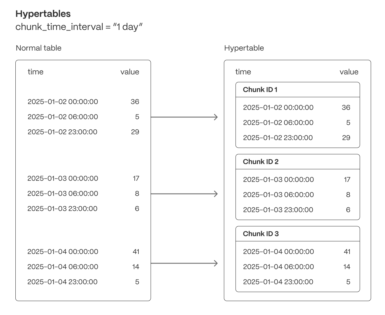
Hypertables are Postgres tables in TimescaleDB that automatically partition your time-series data by time. Time-series data represents the way a system, process, or behavior changes over time. Hypertables enable TimescaleDB to work efficiently with time-series data. Each hypertable is made up of child tables called chunks. Each chunk is assigned a range of time, and only contains data from that range. When you run a query, TimescaleDB identifies the correct chunk and runs the query on it, instead of going through the entire table.

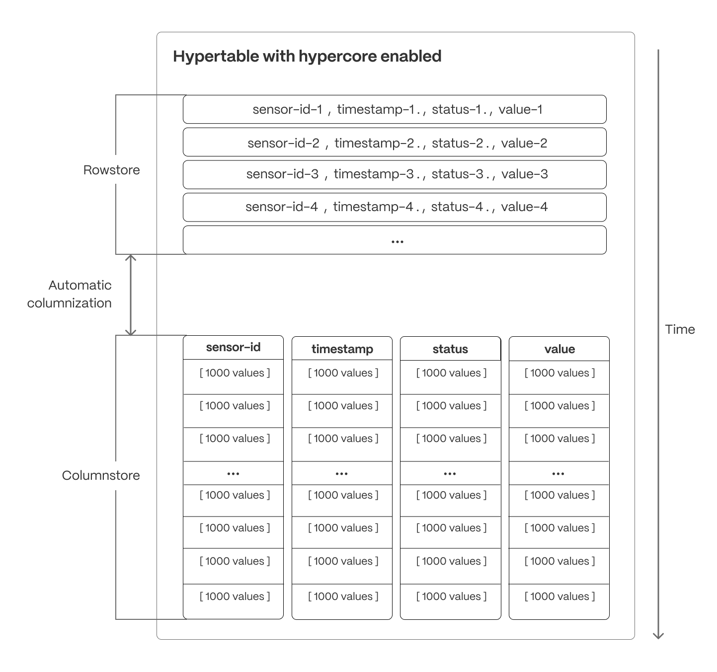
[Hypercore][hypercore] is the hybrid row-columnar storage engine in TimescaleDB used by hypertables. Traditional databases force a trade-off between fast inserts (row-based storage) and efficient analytics (columnar storage). Hypercore eliminates this trade-off, allowing real-time analytics without sacrificing transactional capabilities.

Hypercore dynamically stores data in the most efficient format for its lifecycle:

Row-based storage for recent data: the most recent chunk (and possibly more) is always stored in the rowstore, ensuring fast inserts, updates, and low-latency single record queries. Additionally, row-based storage is used as a writethrough for inserts and updates to columnar storage.
Columnar storage for analytical performance: chunks are automatically compressed into the columnstore, optimizing storage efficiency and accelerating analytical queries.

Unlike traditional columnar databases, hypercore allows data to be inserted or modified at any stage, making it a flexible solution for both high-ingest transactional workloads and real-time analytics—within a single database.

Because TimescaleDB is 100% Postgres, you can use all the standard Postgres tables, indexes, stored procedures, and other objects alongside your hypertables. This makes creating and working with hypertables similar to standard Postgres.

Import time-series data into a hypertable
Unzip nyc_data.tar.gz to a <local folder>.

This test dataset contains historical data from New York's yellow taxi network.

To import up to 100GB of data directly from your current Postgres-based database,

   [migrate with downtime][migrate-with-downtime] using native Postgres tooling. To seamlessly import 100GB-10TB+
   of data, use the [live migration][migrate-live] tooling supplied by Tiger Data. To add data from non-Postgres
   data sources, see [Import and ingest data][data-ingest].

In Terminal, navigate to <local folder> and update the following string with [your connection details][connection-info] to connect to your service.
Create an optimized hypertable for your time-series data:

Create a [hypertable][hypertables-section] with [hypercore][hypercore] enabled by default for your

     time-series data using [CREATE TABLE][hypertable-create-table]. For [efficient queries][secondary-indexes]
     on data in the columnstore, remember to `segmentby` the column you will use most often to filter your data.

In your sql client, run the following command:

If you are self-hosting TimescaleDB v2.19.3 and below, create a [Postgres relational table][pg-create-table], then convert it using [create_hypertable][create_hypertable]. You then enable hypercore with a call to [ALTER TABLE][alter_table_hypercore].

Add another dimension to partition your hypertable more efficiently:
Create an index to support efficient queries by vendor, rate code, and passenger count:
Create Postgres tables for relational data:
Add a table to store the payment types data:
Add a table to store the rates data:
Upload the dataset to your service
Have a quick look at your data

You query hypertables in exactly the same way as you would a relational Postgres table.

Use one of the following SQL editors to run a query and see the data you uploaded:
   - **Data mode**:  write queries, visualize data, and share your results in [Tiger Cloud Console][portal-data-mode] for all your Tiger Cloud services.
   - **SQL editor**: write, fix, and organize SQL faster and more accurately in [Tiger Cloud Console][portal-ops-mode] for a Tiger Cloud service.
   - **psql**: easily run queries on your Tiger Cloud services or self-hosted TimescaleDB deployment from Terminal.

For example:

- Display the number of rides for each fare type:

   This simple query runs in 3 seconds. You see something like:

| rate_code | num_trips |

   |-----------------|-----------|
   |1 |   2266401|
   |2 |     54832|
   |3 |      4126|
   |4 |       967|
   |5 |      7193|
   |6 |        17|
   |99 |        42|

To select all rides taken in the first week of January 2016, and return the total number of trips taken for each rate code:

On this large amount of data, this analytical query on data in the rowstore takes about 59 seconds. You see something like:

| description | num_trips |

   |-----------------|-----------|
   | group ride |   17 |
   | JFK     | 54832 |
   | Nassau or Westchester |    967 |
   | negotiated fare |  7193 |
   | Newark |   4126 |
   | standard rate |    2266401 |

Optimize your data for real-time analytics

When TimescaleDB converts a chunk to the columnstore, it automatically creates a different schema for your data. TimescaleDB creates and uses custom indexes to incorporate the segmentby and orderby parameters when you write to and read from the columstore.

To increase the speed of your analytical queries by a factor of 10 and reduce storage costs by up to 90%, convert data to the columnstore:

Connect to your Tiger Cloud service

In [Tiger Cloud Console][services-portal] open an [SQL editor][in-console-editors]. The in-Console editors display the query speed. You can also connect to your serviceusing [psql][connect-using-psql].

Add a policy to convert chunks to the columnstore at a specific time interval

For example, convert data older than 8 days old to the columstore:

See [add_columnstore_policy][add_columnstore_policy].

The data you imported for this tutorial is from 2016, it was already added to the columnstore by default. However, you get the idea. To see the space savings in action, follow [Try the key Tiger Data features][try-timescale-features].

Just to hit this one home, by converting cooling data to the columnstore, you have increased the speed of your analytical queries by a factor of 10, and reduced storage by up to 90%.

Connect Grafana to Tiger Cloud

To visualize the results of your queries, enable Grafana to read the data in your service:

Log in to Grafana

In your browser, log in to either:

- Self-hosted Grafana: at `http://localhost:3000/`. The default credentials are `admin`, `admin`.
- Grafana Cloud: use the URL and credentials you set when you created your account.

Add your service as a data source
1. Open Connections > Data sources, then click Add new data source.
2. Select PostgreSQL from the list.
3. Configure the connection:
  - Host URL, Database name, Username, and Password

Configure using your [connection details][connection-info]. Host URL is in the format <host>:<port>.

  - `TLS/SSL Mode`: select `require`.
  - `PostgreSQL options`: enable `TimescaleDB`.
  - Leave the default setting for all other fields.

Click Save & test.

Grafana checks that your details are set correctly.

Monitor performance over time

A Grafana dashboard represents a view into the performance of a system, and each dashboard consists of one or more panels, which represent information about a specific metric related to that system.

To visually monitor the volume of taxi rides over time:

Create the dashboard
On the Dashboards page, click New and select New dashboard.
Click Add visualization.
1. Select the data source that connects to your Tiger Cloud service. The Time series visualization is chosen by default.
2. In the Queries section, select Code, then select Time series in Format.
3. Select the data range for your visualization: the data set is from 2016. Click the date range above the panel and set:
  - From:
  - To:
Combine TimescaleDB and Grafana functionality to analyze your data

Combine a TimescaleDB [time_bucket][use-time-buckets], with the Grafana _timefilter() function to set the pickup_datetime column as the filtering range for your visualizations.

This query groups the results by day and orders them by time.

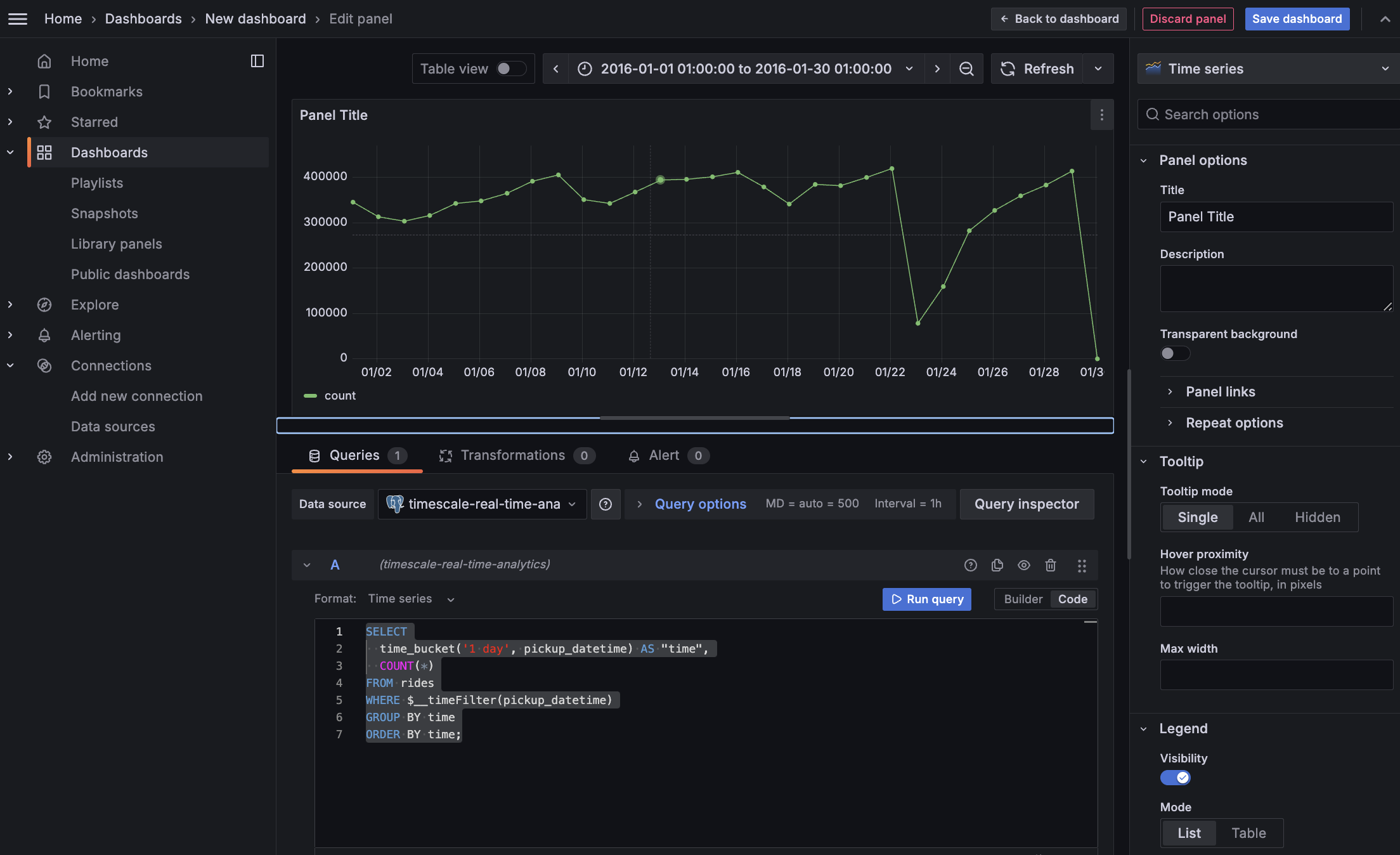
Click Save dashboard

Optimize revenue potential

Having all this data is great but how do you use it? Monitoring data is useful to check what has happened, but how can you analyse this information to your advantage? This section explains how to create a visualization that shows how you can maximize potential revenue.

Set up your data for geospatial queries

To add geospatial analysis to your ride count visualization, you need geospatial data to work out which trips originated where. As TimescaleDB is compatible with all Postgres extensions, use [PostGIS][postgis] to slice data by time and location.

Connect to your [Tiger Cloud service][in-console-editors] and add the PostGIS extension:
Add geometry columns for pick up and drop off locations:
Convert the latitude and longitude points into geometry coordinates that work with PostGIS:

This updates 10,906,860 rows of data on both columns, it takes a while. Coffee is your friend.

Visualize the area where you can make the most money

In this section you visualize a query that returns rides longer than 5 miles for trips taken within 2 km of Times Square. The data includes the distance travelled and is GROUP BY trip_distance and location so that Grafana can plot the data properly.

This enables you to see where a taxi driver is most likely to pick up a passenger who wants a longer ride, and make more money.

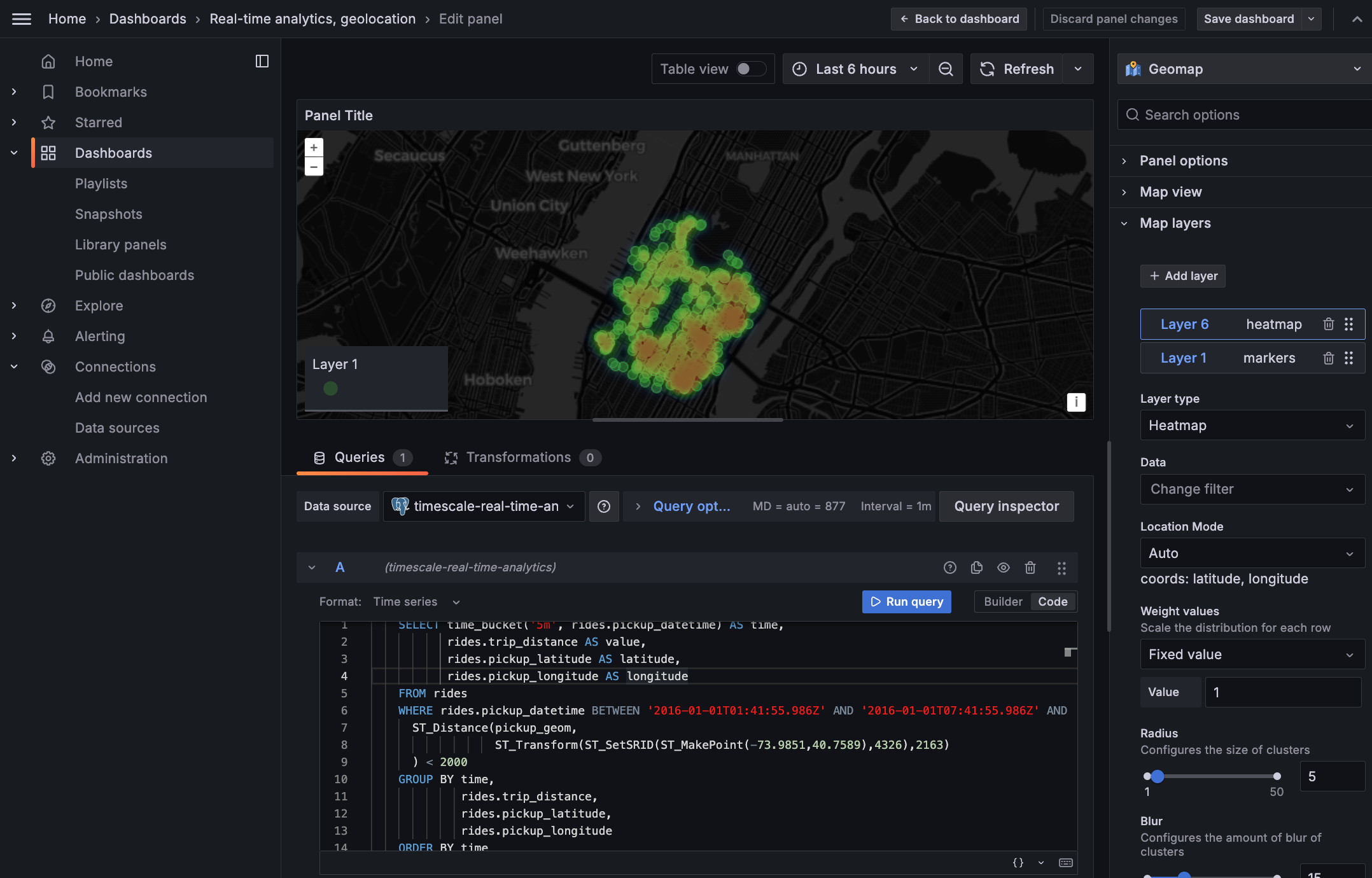
Create a geolocalization dashboard
In Grafana, create a new dashboard that is connected to your Tiger Cloud service data source with a Geomap visualization.
In the Queries section, select Code, then select the Time series Format.

To find rides longer than 5 miles in Manhattan, paste the following query:

You see a world map with a dot on New York.

Zoom into your map to see the visualization clearly.
Customize the visualization
In the Geomap options, under Map Layers, click + Add layer and select Heatmap. You now see the areas where a taxi driver is most likely to pick up a passenger who wants a longer ride, and make more money.

You have integrated Grafana with a Tiger Cloud service and made insights based on visualization of your data.

===== PAGE: https://docs.tigerdata.com/tutorials/real-time-analytics-energy-consumption/ =====

Examples:

Example 1 (bash):

psql -d "postgres://<username>:<password>@<host>:<port>/<database-name>?sslmode=require"

Example 2 (sql):

CREATE TABLE "rides"(
               vendor_id TEXT,
               pickup_datetime TIMESTAMP WITHOUT TIME ZONE NOT NULL,
               dropoff_datetime TIMESTAMP WITHOUT TIME ZONE NOT NULL,
               passenger_count NUMERIC,
               trip_distance NUMERIC,
               pickup_longitude  NUMERIC,
               pickup_latitude   NUMERIC,
               rate_code         INTEGER,
               dropoff_longitude NUMERIC,
               dropoff_latitude  NUMERIC,
               payment_type INTEGER,
               fare_amount NUMERIC,
               extra NUMERIC,
               mta_tax NUMERIC,
               tip_amount NUMERIC,
               tolls_amount NUMERIC,
               improvement_surcharge NUMERIC,
               total_amount NUMERIC
             ) WITH (
               tsdb.hypertable,
               tsdb.partition_column='pickup_datetime',
               tsdb.create_default_indexes=false,
               tsdb.segmentby='vendor_id',
               tsdb.orderby='pickup_datetime DESC'
             );

Example 3 (sql):

SELECT add_dimension('rides', by_hash('payment_type', 2));

Example 4 (sql):

CREATE INDEX ON rides (vendor_id, pickup_datetime DESC);
             CREATE INDEX ON rides (rate_code, pickup_datetime DESC);
             CREATE INDEX ON rides (passenger_count, pickup_datetime DESC);

variance_y() | variance_x()

URL: llms-txt#variance_y()-|-variance_x()

===== PAGE: https://docs.tigerdata.com/api/_hyperfunctions/stats_agg-two-variables/skewness_y_x/ =====

approx_percentile()

URL: llms-txt#approx_percentile()

===== PAGE: https://docs.tigerdata.com/api/_hyperfunctions/uddsketch/num_vals/ =====

sum()

URL: llms-txt#sum()

===== PAGE: https://docs.tigerdata.com/api/_hyperfunctions/stats_agg-one-variable/stats_agg/ =====

sum_y() | sum_x()

URL: llms-txt#sum_y()-|-sum_x()

===== PAGE: https://docs.tigerdata.com/api/_hyperfunctions/stats_agg-two-variables/kurtosis_y_x/ =====

About TimescaleDB hyperfunctions

URL: llms-txt#about-timescaledb-hyperfunctions

Contents:

Available hyperfunctions
Function pipelines
Toolkit feature development
Contribute to TimescaleDB Toolkit

TimescaleDB hyperfunctions are a specialized set of functions that power real-time analytics on time series and events. IoT devices, IT systems, marketing analytics, user behavior, financial metrics, cryptocurrency - these are only a few examples of domains where hyperfunctions can make a huge difference. Hyperfunctions provide you with meaningful, actionable insights in real time.

Tiger Cloud includes all hyperfunctions by default, while self-hosted TimescaleDB includes a subset of them. For additional hyperfunctions, install the [TimescaleDB Toolkit][install-toolkit] Postgres extension.

Available hyperfunctions

Here is a list of all the hyperfunctions provided by TimescaleDB. Hyperfunctions with a tick in the Toolkit column require an installation of TimescaleDB Toolkit for self-hosted deployments. Hyperfunctions with a tick in the Experimental column are still under development.

Experimental features could have bugs. They might not be backwards compatible, and could be removed in future releases. Use these features at your own risk, and do not use any experimental features in production.

When you upgrade the timescaledb extension, the experimental schema is removed by default. To use experimental features after an upgrade, you need to add the experimental schema again.

<HyperfunctionTable

includeExperimental

For more information about each of the API calls listed in this table, see the [hyperfunction API documentation][api-hyperfunctions].

Function pipelines

Function pipelines are an experimental feature, designed to radically improve the developer ergonomics of analyzing data in Postgres and SQL, by applying principles from functional programming and popular tools like Python's Pandas, and PromQL.

SQL is the best language for data analysis, but it is not perfect, and at times can get quite unwieldy. For example, this query gets data from the last day from the measurements table, sorts the data by the time column, calculates the delta between the values, takes the absolute value of the delta, and then takes the sum of the result of the previous steps:

You can express the same query with a function pipeline like this:

Function pipelines are completely SQL compliant, meaning that any tool that speaks SQL is able to support data analysis using function pipelines.

For more information about how function pipelines work, read our [blog post][blog-function-pipelines].

Toolkit feature development

TimescaleDB Toolkit features are developed in the open. As features are developed they are categorized as experimental, beta, stable, or deprecated. This documentation covers the stable features, but more information on our experimental features in development can be found in the [Toolkit repository][gh-docs].

Contribute to TimescaleDB Toolkit

We want and need your feedback! What are the frustrating parts of analyzing time-series data? What takes far more code than you feel it should? What runs slowly, or only runs quickly after many rewrites? We want to solve community-wide problems and incorporate as much feedback as possible.

Join the [discussion][gh-discussions].
Check out the [proposed features][gh-proposed].
Explore the current [feature requests][gh-requests].
Add your own [feature request][gh-newissue].

===== PAGE: https://docs.tigerdata.com/use-timescale/hyperfunctions/approx-count-distincts/ =====

Examples:

Example 1 (SQL):

SELECT device id,
sum(abs_delta) as volatility
FROM (
 SELECT device_id,
abs(val - lag(val) OVER last_day) as abs_delta
FROM measurements
WHERE ts >= now()-'1 day'::interval) calc_delta
GROUP BY device_id;

Example 2 (SQL):

SELECT device_id,
 timevector(ts, val) -> sort() -> delta() -> abs() -> sum() as volatility
FROM measurements
WHERE ts >= now()-'1 day'::interval
GROUP BY device_id;

kurtosis()

URL: llms-txt#kurtosis()

===== PAGE: https://docs.tigerdata.com/api/_hyperfunctions/stats_agg-one-variable/num_vals/ =====

num_vals()

URL: llms-txt#num_vals()

===== PAGE: https://docs.tigerdata.com/api/_hyperfunctions/uddsketch/intro/ =====

Estimate the value at a given percentile, or the percentile rank of a given value, using the UddSketch algorithm. This estimation is more memory- and CPU-efficient than an exact calculation using Postgres's percentile_cont and percentile_disc functions.

uddsketch is one of two advanced percentile approximation aggregates provided in TimescaleDB Toolkit. It produces stable estimates within a guaranteed relative error.

The other advanced percentile approximation aggregate is [tdigest][tdigest], which is more accurate at extreme quantiles, but is somewhat dependent on input order.

If you aren't sure which aggregate to use, try the default percentile estimation method, [percentile_agg][percentile_agg]. It uses the uddsketch algorithm with some sensible defaults.

For more information about percentile approximation algorithms, see the [algorithms overview][algorithms].

===== PAGE: https://docs.tigerdata.com/api/_hyperfunctions/uddsketch/approx_percentile_rank/ =====

Last observation carried forward

URL: llms-txt#last-observation-carried-forward

Last observation carried forward (LOCF) is a form of linear interpolation used to fill gaps in your data. It takes the last known value and uses it as a replacement for the missing data.

For more information about gapfilling and interpolation API calls, see the [hyperfunction API documentation][hyperfunctions-api-gapfilling].

===== PAGE: https://docs.tigerdata.com/use-timescale/hyperfunctions/stats-aggs/ =====

kurtosis_y() | kurtosis_x()

URL: llms-txt#kurtosis_y()-|-kurtosis_x()

===== PAGE: https://docs.tigerdata.com/api/_hyperfunctions/stats_agg-two-variables/x_intercept/ =====

average_y() | average_x()

URL: llms-txt#average_y()-|-average_x()

===== PAGE: https://docs.tigerdata.com/api/_hyperfunctions/stats_agg-two-variables/intercept/ =====

Real-time analytics with Tiger Cloud and Grafana

URL: llms-txt#real-time-analytics-with-tiger-cloud-and-grafana

Contents:

Prerequisites
Optimize time-series data in hypertables
Optimize your data for real-time analytics
Write fast analytical queries
Connect Grafana to Tiger Cloud
Visualize energy consumption

Energy providers understand that customers tend to lose patience when there is not enough power for them to complete day-to-day activities. Task one is keeping the lights on. If you are transitioning to renewable energy, it helps to know when you need to produce energy so you can choose a suitable energy source.

Real-time analytics refers to the process of collecting, analyzing, and interpreting data instantly as it is generated. This approach enables you to track and monitor activity, make the decisions based on real-time insights on data stored in a Tiger Cloud service and keep those lights on.

[Grafana][grafana-docs] is a popular data visualization tool that enables you to create customizable dashboards and effectively monitor your systems and applications.

This page shows you how to integrate Grafana with a Tiger Cloud service and make insights based on visualization of data optimized for size and speed in the columnstore.

To follow the steps on this page:

Create a target [Tiger Cloud service][create-service] with the Real-time analytics capability.

You need [your connection details][connection-info]. This procedure also works for [self-hosted TimescaleDB][enable-timescaledb].

Install and run [self-managed Grafana][grafana-self-managed], or sign up for [Grafana Cloud][grafana-cloud].

Optimize time-series data in hypertables

Hypercore dynamically stores data in the most efficient format for its lifecycle:

Row-based storage for recent data: the most recent chunk (and possibly more) is always stored in the rowstore, ensuring fast inserts, updates, and low-latency single record queries. Additionally, row-based storage is used as a writethrough for inserts and updates to columnar storage.
Columnar storage for analytical performance: chunks are automatically compressed into the columnstore, optimizing storage efficiency and accelerating analytical queries.

Import time-series data into a hypertable
Unzip metrics.csv.gz to a <local folder>.

This test dataset contains energy consumption data.

To import up to 100GB of data directly from your current Postgres based database,

   [migrate with downtime][migrate-with-downtime] using native Postgres tooling. To seamlessly import 100GB-10TB+
   of data, use the [live migration][migrate-live] tooling supplied by Tiger Data. To add data from non-Postgres
   data sources, see [Import and ingest data][data-ingest].

In Terminal, navigate to <local folder> and update the following string with [your connection details][connection-info] to connect to your service.
Create an optimized hypertable for your time-series data:

Create a [hypertable][hypertables-section] with [hypercore][hypercore] enabled by default for your

  time-series data using [CREATE TABLE][hypertable-create-table]. For [efficient queries][secondary-indexes]
  on data in the columnstore, remember to `segmentby` the column you will use most often to filter your data.

In your sql client, run the following command:

Upload the dataset to your service
Have a quick look at your data

You query hypertables in exactly the same way as you would a relational Postgres table.

Use one of the following SQL editors to run a query and see the data you uploaded:
   - **Data mode**:  write queries, visualize data, and share your results in [Tiger Cloud Console][portal-data-mode] for all your Tiger Cloud services.
   - **SQL editor**: write, fix, and organize SQL faster and more accurately in [Tiger Cloud Console][portal-ops-mode] for a Tiger Cloud service.
   - **psql**: easily run queries on your Tiger Cloud services or self-hosted TimescaleDB deployment from Terminal.

On this amount of data, this query on data in the rowstore takes about 3.6 seconds. You see something like:

| Time | value |

|------------------------------|-------|
| 2023-05-29 22:00:00+00 | 23.1  |
| 2023-05-28 22:00:00+00 | 19.5  |
| 2023-05-30 22:00:00+00 | 25    |
| 2023-05-31 22:00:00+00 | 8.1   |

Optimize your data for real-time analytics

To increase the speed of your analytical queries by a factor of 10 and reduce storage costs by up to 90%, convert data to the columnstore:

Connect to your Tiger Cloud service

Add a policy to convert chunks to the columnstore at a specific time interval

For example, 60 days after the data was added to the table:

See [add_columnstore_policy][add_columnstore_policy].

Faster analytical queries on data in the columnstore

Now run the analytical query again:

On this amount of data, this analytical query on data in the columnstore takes about 250ms.

Just to hit this one home, by converting cooling data to the columnstore, you have increased the speed of your analytical queries by a factor of 10, and reduced storage by up to 90%.

Write fast analytical queries

Aggregation is a way of combining data to get insights from it. Average, sum, and count are all examples of simple aggregates. However, with large amounts of data aggregation slows things down, quickly. Continuous aggregates are a kind of hypertable that is refreshed automatically in the background as new data is added, or old data is modified. Changes to your dataset are tracked, and the hypertable behind the continuous aggregate is automatically updated in the background.

By default, querying continuous aggregates provides you with real-time data. Pre-aggregated data from the materialized view is combined with recent data that hasn't been aggregated yet. This gives you up-to-date results on every query.

You create continuous aggregates on uncompressed data in high-performance storage. They continue to work on [data in the columnstore][test-drive-enable-compression] and [rarely accessed data in tiered storage][test-drive-tiered-storage]. You can even create [continuous aggregates on top of your continuous aggregates][hierarchical-caggs].

Monitor energy consumption on a day-to-day basis
Create a continuous aggregate kwh_day_by_day for energy consumption:
Add a refresh policy to keep kwh_day_by_day up-to-date:
Monitor energy consumption on an hourly basis
Create a continuous aggregate kwh_hour_by_hour for energy consumption:
Add a refresh policy to keep the continuous aggregate up-to-date:
Analyze your data

Now you have made continuous aggregates, it could be a good idea to use them to perform analytics on your data.

For example, to see how average energy consumption changes during weekdays over the last year, run the following query:

You see something like:

| day | ordinal | value |

  | --- | ------- | ----- |
  | Mon | 2 | 23.08078714975423 |
  | Sun | 1 | 19.511430831944395 |
  | Tue | 3 | 25.003118897837307 |
  | Wed | 4 | 8.09300571759772 |

Connect Grafana to Tiger Cloud

To visualize the results of your queries, enable Grafana to read the data in your service:

Log in to Grafana

In your browser, log in to either:

- Self-hosted Grafana: at `http://localhost:3000/`. The default credentials are `admin`, `admin`.
- Grafana Cloud: use the URL and credentials you set when you created your account.

Add your service as a data source
1. Open Connections > Data sources, then click Add new data source.
2. Select PostgreSQL from the list.
3. Configure the connection:
  - Host URL, Database name, Username, and Password

Configure using your [connection details][connection-info]. Host URL is in the format <host>:<port>.

  - `TLS/SSL Mode`: select `require`.
  - `PostgreSQL options`: enable `TimescaleDB`.
  - Leave the default setting for all other fields.

Click Save & test.

Grafana checks that your details are set correctly.

Visualize energy consumption

A Grafana dashboard represents a view into the performance of a system, and each dashboard consists of one or more panels, which represent information about a specific metric related to that system.

To visually monitor the volume of energy consumption over time:

Create the dashboard
On the Dashboards page, click New and select New dashboard.
Click Add visualization, then select the data source that connects to your Tiger Cloud service and the Bar chart visualization.

In the Queries section, select Code, then run the following query based on your continuous aggregate:

This query averages the results for households in a specific time zone by hour and orders them by time.

  Because you use a continuous aggregate, this data is always correct in real time.

You see that energy consumption is highest in the evening and at breakfast time. You also know that the wind

  drops off in the evening. This data proves that you need to supply a supplementary power source for peak times,
  or plan to store energy during the day for peak times.

Click Save dashboard

You have integrated Grafana with a Tiger Cloud service and made insights based on visualization of your data.

===== PAGE: https://docs.tigerdata.com/tutorials/simulate-iot-sensor-data/ =====

Examples:

Example 1 (bash):

psql -d "postgres://<username>:<password>@<host>:<port>/<database-name>?sslmode=require"

Example 2 (sql):

CREATE TABLE "metrics"(
               created timestamp with time zone default now() not null,
               type_id integer                                not null,
               value   double precision                       not null
             ) WITH (
               tsdb.hypertable,
               tsdb.partition_column='created',
               tsdb.segmentby = 'type_id',
               tsdb.orderby = 'created DESC'
             );

Example 3 (sql):

\COPY metrics FROM metrics.csv CSV;

Example 4 (sql):

SELECT time_bucket('1 day', created, 'Europe/Berlin') AS "time",
    round((last(value, created) - first(value, created)) * 100.) / 100. AS value
    FROM metrics
    WHERE type_id = 5
    GROUP BY 1;

stats_agg() (one variable)

URL: llms-txt#stats_agg()-(one-variable)

===== PAGE: https://docs.tigerdata.com/api/_hyperfunctions/stats_agg-one-variable/average/ =====

rollup()

URL: llms-txt#rollup()

===== PAGE: https://docs.tigerdata.com/api/_hyperfunctions/uddsketch/approx_percentile_array/ =====

Percentile approximation

URL: llms-txt#percentile-approximation

In general, percentiles are useful for understanding the distribution of data. The fiftieth percentile is the point at which half of your data is greater and half is lesser. The tenth percentile is the point at which 90% of the data is greater, and 10% is lesser. The ninety-ninth percentile is the point at which 1% is greater, and 99% is lesser.

The fiftieth percentile, or median, is often a more useful measure than the average, especially when your data contains outliers. Outliers can dramatically change the average, but do not affect the median as much. For example, if you have three rooms in your house and two of them are 40℉ (4℃) and one is 130℉ (54℃), the average room temperature is 70℉ (21℃), which doesn't tell you much. However, the fiftieth percentile temperature is 40℉ (4℃), which tells you that at least half your rooms are at refrigerator temperatures (also, you should probably get your heating checked!)

Percentiles are sometimes avoided because calculating them requires more CPU and memory than an average or other aggregate measures. This is because an exact computation of the percentile needs the full dataset as an ordered list. TimescaleDB uses approximation algorithms to calculate a percentile without requiring all of the data. This also makes them more compatible with continuous aggregates. By default, TimescaleDB uses uddsketch, but you can also choose to use tdigest. For more information about these algorithms, see the [advanced aggregation methods][advanced-agg] documentation.

Technically, a percentile divides a group into 100 equally sized pieces, while a quantile divides a group into an arbitrary number of pieces. Because we don't always use exactly 100 buckets, "quantile" is the more technically correct term in this case. However, we use the word "percentile" because it's a more common word for this type of function.

For more information about how percentile approximation works, read our [percentile approximation blog][blog-percentile-approx].
For more information about percentile approximation API calls, see the [hyperfunction API documentation][hyperfunctions-api-approx-percentile].

===== PAGE: https://docs.tigerdata.com/use-timescale/hyperfunctions/advanced-agg/ =====

stats_agg() (two variables)

URL: llms-txt#stats_agg()-(two-variables)

===== PAGE: https://docs.tigerdata.com/api/_hyperfunctions/stats_agg-two-variables/average_y_x/ =====

skewness()

URL: llms-txt#skewness()

===== PAGE: https://docs.tigerdata.com/api/_hyperfunctions/stats_agg-one-variable/rolling/ =====

rolling()

URL: llms-txt#rolling()

===== PAGE: https://docs.tigerdata.com/api/_hyperfunctions/stats_agg-two-variables/slope/ =====

uddsketch()

URL: llms-txt#uddsketch()

===== PAGE: https://docs.tigerdata.com/api/_hyperfunctions/uddsketch/percentile_agg/ =====

determination_coeff()

URL: llms-txt#determination_coeff()

===== PAGE: https://docs.tigerdata.com/api/_hyperfunctions/stats_agg-two-variables/variance_y_x/ =====

approx_percentile_array()

URL: llms-txt#approx_percentile_array()

===== PAGE: https://docs.tigerdata.com/api/_hyperfunctions/counter_agg/delta/ =====

Tiger Data architecture for real-time analytics

URL: llms-txt#tiger-data-architecture-for-real-time-analytics

Contents:

Introduction
- What is real-time analytics?
- Tiger Cloud: real-time analytics from Postgres
Data model
- Efficient data partitioning
- Row-columnar storage
- Columnar storage layout
- Data mutability
Query optimizations
- Skip unnecessary data

Tiger Data has created a powerful application database for real-time analytics on time-series data. It integrates seamlessly with the Postgres ecosystem and enhances it with automatic time-based partitioning, hybrid row-columnar storage, and vectorized execution—enabling high-ingest performance, sub-second queries, and full SQL support at scale.

Tiger Cloud offers managed database services that provide a stable and reliable environment for your applications. Each service is based on a Postgres database instance and the TimescaleDB extension.

By making use of incrementally updated materialized views and advanced analytical functions, TimescaleDB reduces compute overhead and improves query efficiency. Developers can continue using familiar SQL workflows and tools, while benefiting from a database purpose-built for fast, scalable analytics.

This document outlines the architectural choices and optimizations that power TimescaleDB and Tiger Cloud’s performance and scalability while preserving Postgres’s reliability and transactional guarantees.

Want to read this whitepaper from the comfort of your own computer?

Tiger Data architecture for real-time analytics (PDF)

What is real-time analytics?

Real-time analytics enables applications to process and query data as it is generated and as it accumulates, delivering immediate and ongoing insights for decision-making. Unlike traditional analytics, which relies on batch processing and delayed reporting, real-time analytics supports both instant queries on fresh data and fast exploration of historical trends—powering applications with sub-second query performance across vast, continuously growing datasets.

Many modern applications depend on real-time analytics to drive critical functionality:

IoT monitoring systems track sensor data over time, identifying long-term performance patterns while still surfacing anomalies as they arise. This allows businesses to optimize maintenance schedules, reduce costs, and improve reliability.
Financial and business intelligence platforms analyze both current and historical data to detect trends, assess risk, and uncover opportunities—from tracking stock performance over a day, week, or year to identifying spending patterns across millions of transactions.
Interactive customer dashboards empower users to explore live and historical data in a seamless experience—whether it's a SaaS product providing real-time analytics on business operations, a media platform analyzing content engagement, or an e-commerce site surfacing personalized recommendations based on recent and past behavior.

Real-time analytics isn't just about reacting to the latest data, although that is critically important. It's also about delivering fast, interactive, and scalable insights across all your data, enabling better decision-making and richer user experiences. Unlike traditional ad-hoc analytics used by analysts, real-time analytics powers applications—driving dynamic dashboards, automated decisions, and user-facing insights at scale.

To achieve this, real-time analytics systems must meet several key requirements:

Low-latency queries ensure sub-second response times even under high load, enabling fast insights for dashboards, monitoring, and alerting.
Low-latency ingest minimizes the lag between when data is created and when it becomes available for analysis, ensuring fresh and accurate insights.
Data mutability allows for efficient updates, corrections, and backfills, ensuring analytics reflect the most accurate state of the data.
Concurrency and scalability enable systems to handle high query volumes and growing workloads without degradation in performance.
Seamless access to both recent and historical data ensures fast queries across time, whether analyzing live, streaming data, or running deep historical queries on days or months of information.
Query flexibility provides full SQL support, allowing for complex queries with joins, filters, aggregations, and analytical functions.

Tiger Cloud: real-time analytics from Postgres

Tiger Cloud is a high-performance database that brings real-time analytics to applications. It combines fast queries, high ingest performance, and full SQL support—all while ensuring scalability and reliability. Tiger Cloud extends Postgres with the TimescaleDB extension. It enables sub-second queries on vast amounts of incoming data while providing optimizations designed for continuously updating datasets.

Tiger Cloud achieves this through the following optimizations:

Efficient data partitioning: automatically and transparently partitioning data into chunks, ensuring fast queries, minimal indexing overhead, and seamless scalability
Row-columnar storage: providing the flexibility of a row store for transactions and the performance of a column store for analytics
**Optimized query execution: **using techniques like chunk and batch exclusion, columnar storage, and vectorized execution to minimize latency
Continuous aggregates: precomputing analytical results for fast insights without expensive reprocessing
**Cloud-native operation: **compute/compute separation, elastic usage-based storage, horizontal scale out, data tiering to object storage
**Operational simplicity: **offering high availability, connection pooling, and automated backups for reliable and scalable real-time applications

With Tiger Cloud, developers can build low-latency, high-concurrency applications that seamlessly handle streaming data, historical queries, and real-time analytics while leveraging the familiarity and power of Postgres.

Today's applications demand a database that can handle real-time analytics and transactional queries without sacrificing speed, flexibility, or SQL compatibility (including joins between tables). TimescaleDB achieves this with hypertables, which provide an automatic partitioning engine, and hypercore, a hybrid row-columnar storage engine designed to deliver high-performance queries and efficient compression (up to 95%) within Postgres.

Efficient data partitioning

TimescaleDB provides hypertables, a table abstraction that automatically partitions data into chunks in real time (using time stamps or incrementing IDs) to ensure fast queries and predictable performance as datasets grow. Unlike traditional relational databases that require manual partitioning, hypertables automate all aspects of partition management, keeping locking minimal even under high ingest load.

At ingest time, hypertables ensure that Postgres can deal with a constant stream of data without suffering from table bloat and index degradation by automatically partitioning data across time. Because each chunk is ordered by time and has its own indexes and storage, writes are usually isolated to small, recent chunks—keeping index sizes small, improving cache locality, and reducing the overhead of vacuum and background maintenance operations. This localized write pattern minimizes write amplification and ensures consistently high ingest performance, even as total data volume grows.

At query time, hypertables efficiently exclude irrelevant chunks from the execution plan when the partitioning column is used in a WHERE clause. This architecture ensures fast query execution, avoiding the gradual slowdowns that affect non-partitioned tables as they accumulate millions of rows. Chunk-local indexes keep indexing overhead minimal, ensuring index operations scans remain efficient regardless of dataset size.

Hypertables are the foundation for all of TimescaleDB’s real-time analytics capabilities. They enable seamless data ingestion, high-throughput writes, optimized query execution, and chunk-based lifecycle management—including automated data retention (drop a chunk) and data tiering (move a chunk to object storage).

Row-columnar storage

Traditional databases force a trade-off between fast inserts (row-based storage) and efficient analytics (columnar storage). Hypercore eliminates this trade-off, allowing real-time analytics without sacrificing transactional capabilities.

Hypercore dynamically stores data in the most efficient format for its lifecycle:

Row-based storage for recent data: the most recent chunk (and possibly more) is always stored in the rowstore, ensuring fast inserts, updates, and low-latency single record queries. Additionally, row-based storage is used as a writethrough for inserts and updates to columnar storage.
Columnar storage for analytical performance: chunks are automatically compressed into the columnstore, optimizing storage efficiency and accelerating analytical queries.

Columnar storage layout

TimescaleDB’s columnar storage layout optimizes analytical query performance by structuring data efficiently on disk, reducing scan times, and maximizing compression rates. Unlike traditional row-based storage, where data is stored sequentially by row, columnar storage organizes and compresses data by column, allowing queries to retrieve only the necessary fields in batches rather than scanning entire rows. But unlike many column store implementations, TimescaleDB’s columnstore supports full mutability—inserts, upserts, updates, and deletes, even at the individual record level—with transactional guarantees. Data is also immediately visible to queries as soon as it is written.

Columnar batches

TimescaleDB uses columnar collocation and columnar compression within row-based storage to optimize analytical query performance while maintaining full Postgres compatibility. This approach ensures efficient storage, high compression ratios, and rapid query execution.

A rowstore chunk is converted to a columnstore chunk by successfully grouping together sets of rows (typically up to 1000) into a single batch, then converting the batch into columnar form.

Each compressed batch does the following:

Encapsulates columnar data in compressed arrays of up to 1,000 values per column, stored as a single entry in the underlying compressed table
Uses a column-major format within the batch, enabling efficient scans by co-locating values of the same column and allowing the selection of individual columns without reading the entire batch
Applies advanced compression techniques at the column level, including run-length encoding, delta encoding, and Gorilla compression, to significantly reduce storage footprint (by up to 95%) and improve I/O performance.

While the chunk interval of rowstore and columnstore batches usually remains the same, TimescaleDB can also combine columnstore batches so they use a different chunk interval.

This architecture provides the benefits of columnar storage—optimized scans, reduced disk I/O, and improved analytical performance—while seamlessly integrating with Postgres’s row-based execution model.

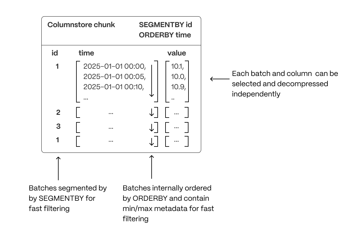
Segmenting and ordering data

To optimize query performance, TimescaleDB allows explicit control over how data is physically organized within columnar storage. By structuring data effectively, queries can minimize disk reads and execute more efficiently, using vectorized execution for parallel batch processing where possible.

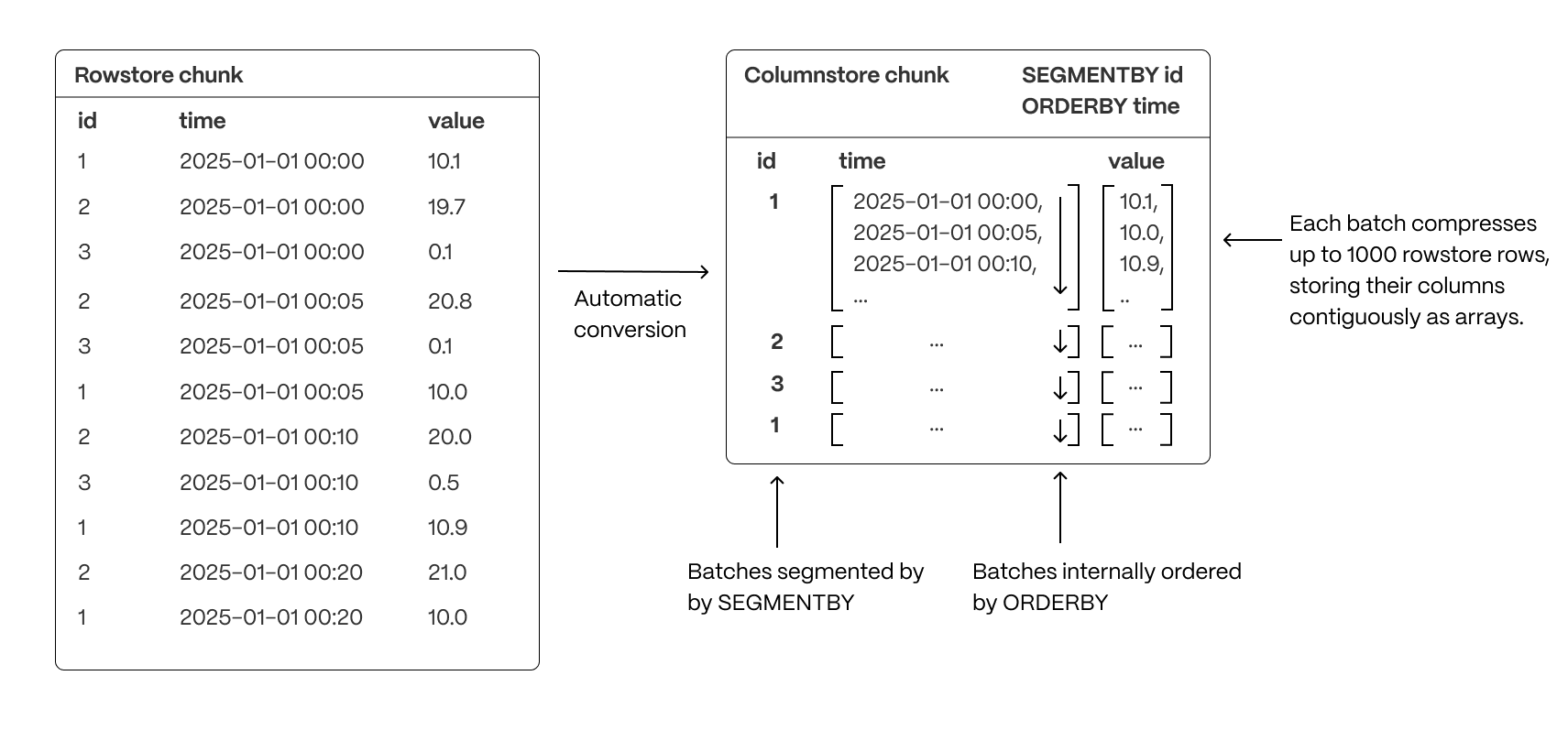
Group related data together to improve scan efficiency: organizing rows into logical segments ensures that queries filtering by a specific value only scan relevant data sections. For example, in the above, querying for a specific ID is particularly fast. (Implemented with SEGMENTBY.)
Sort data within segments to accelerate range queries: defining a consistent order reduces the need for post-query sorting, making time-based queries and range scans more efficient. (Implemented with ORDERBY.)
Reduce disk reads and maximize vectorized execution: a well-structured storage layout enables efficient batch processing (Single Instruction, Multiple Data, or SIMD vectorization) and parallel execution, optimizing query performance.

By combining segmentation and ordering, TimescaleDB ensures that columnar queries are not only fast but also resource-efficient, enabling high-performance real-time analytics.

Traditional databases force a trade-off between fast updates and efficient analytics. Fully immutable storage is impractical in real-world applications, where data needs to change. Asynchronous mutability—where updates only become visible after batch processing—introduces delays that break real-time workflows. In-place mutability, while theoretically ideal, is prohibitively slow in columnar storage, requiring costly decompression, segmentation, ordering, and recompression cycles.

Hypercore navigates these trade-offs with a hybrid approach that enables immediate updates without modifying compressed columnstore data in place. By staging changes in an interim rowstore chunk, hypercore allows updates and deletes to happen efficiently while preserving the analytical performance of columnar storage.

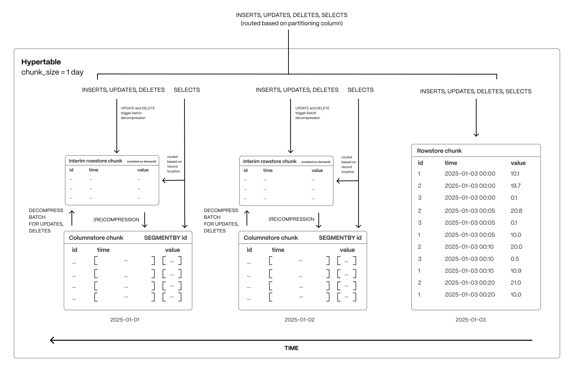
Real-time writes without delays

All new data which is destined for a columnstore chunk is first written to an interim rowstore chunk, ensuring high-speed ingestion and immediate queryability. Unlike fully columnar systems that require ingestion to go through compression pipelines, hypercore allows fresh data to remain in a fast row-based structure before being later compressed into columnar format in ordered batches as normal.

Queries transparently access both the rowstore and columnstore chunks, meaning applications always see the latest data instantly, regardless of its storage format.

Efficient updates and deletes without performance penalties

When modifying or deleting existing data, hypercore avoids the inefficiencies of both asynchronous updates and in-place modifications. Instead of modifying compressed storage directly, affected batches are decompressed and staged in the interim rowstore chunk, where changes are applied immediately.

These modified batches remain in row storage until they are recompressed and reintegrated into the columnstore (which happens automatically via a background process). This approach ensures updates are immediately visible, but without the expensive overhead of decompressing and rewriting entire chunks. This approach avoids:

The rigidity of immutable storage, which requires workarounds like versioning or copy-on-write strategies
The delays of asynchronous updates, where modified data is only visible after batch processing
The performance hit of in-place mutability, which makes compressed storage prohibitively slow for frequent updates
The restrictions some databases have on not altering the segmentation or ordering keys

Query optimizations

Real-time analytics isn’t just about raw speed—it’s about executing queries efficiently, reducing unnecessary work, and maximizing performance. TimescaleDB optimizes every step of the query lifecycle to ensure that queries scan only what’s necessary, make use of data locality, and execute in parallel for sub-second response times over large datasets.

Skip unnecessary data

TimescaleDB minimizes the amount of data a query touches, reducing I/O and improving execution speed:

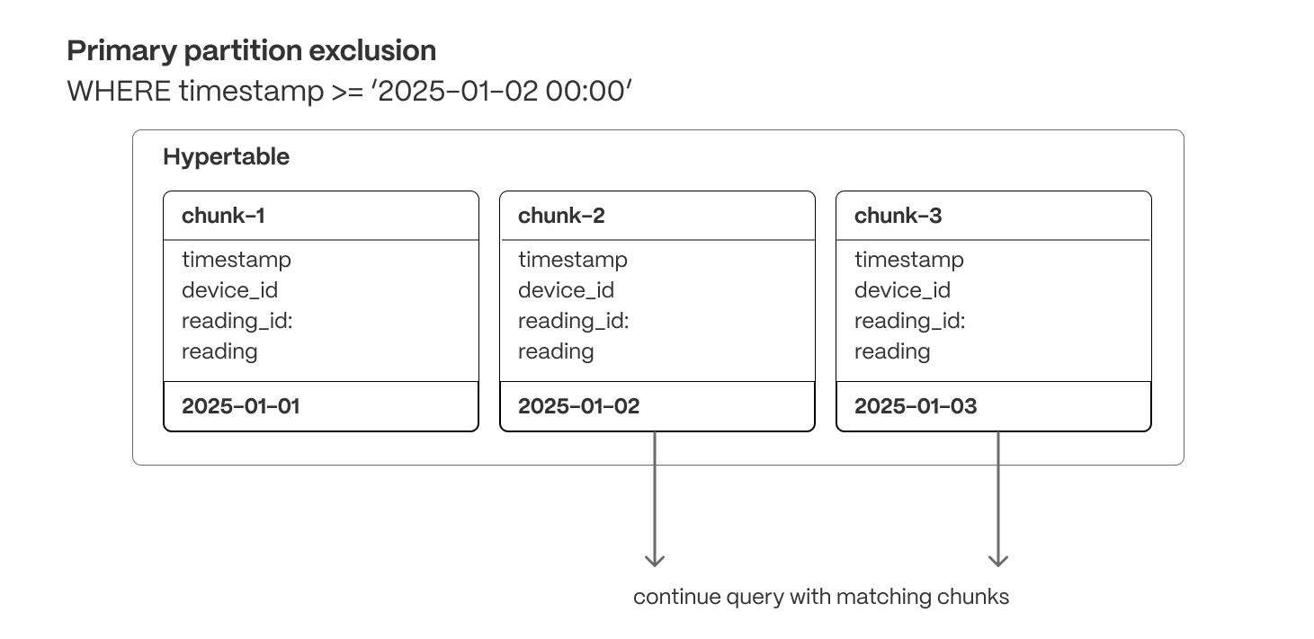
Primary partition exclusion (row and columnar)

Queries automatically skip irrelevant partitions (chunks) based on the primary partitioning key (usually a timestamp), ensuring they only scan relevant data.

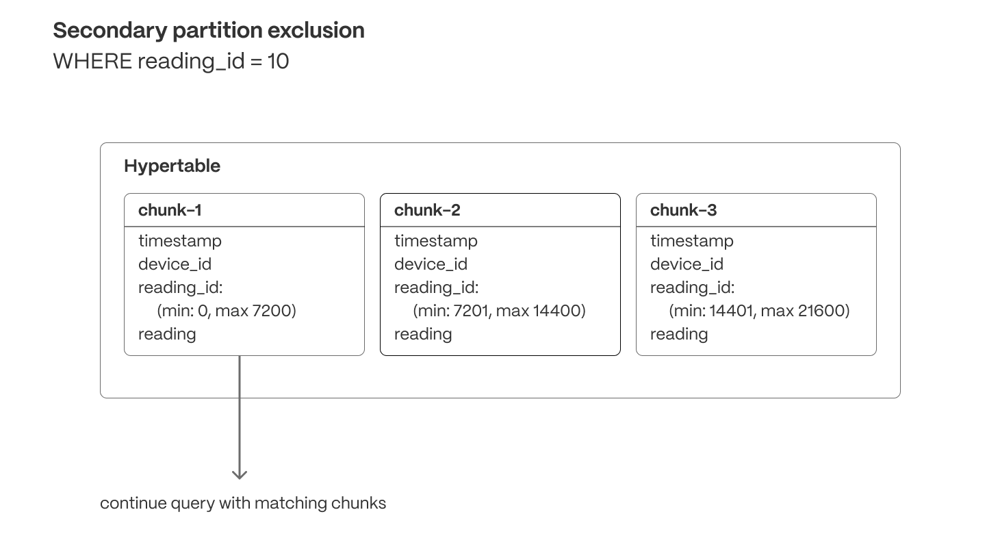
Secondary partition exclusion (columnar)

Min/max metadata allows queries filtering on correlated dimensions (e.g., order_id or secondary timestamps) to exclude chunks that don’t contain relevant data.

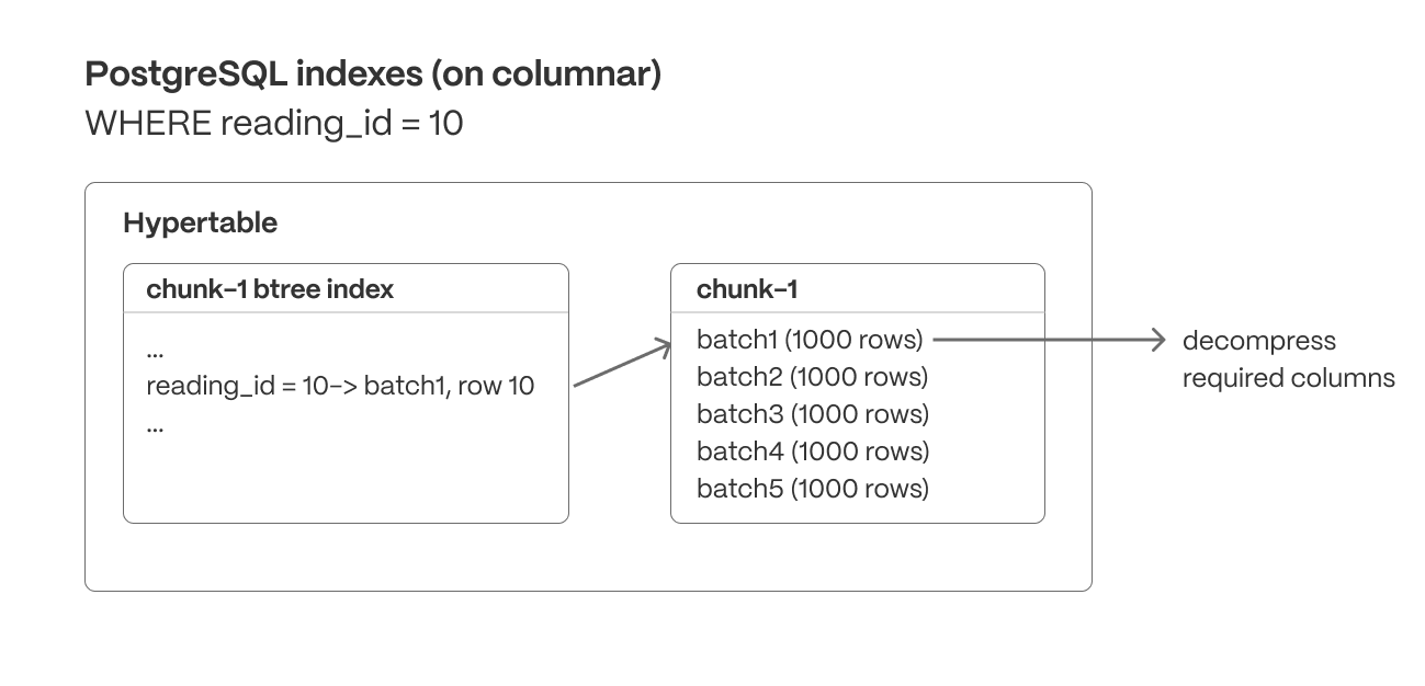
Postgres indexes (row and columnar)

Unlike many databases, TimescaleDB supports sparse indexes on columnstore data, allowing queries to efficiently locate specific values within both row-based and compressed columnar storage. These indexes enable fast lookups, range queries, and filtering operations that further reduce unnecessary data scans.

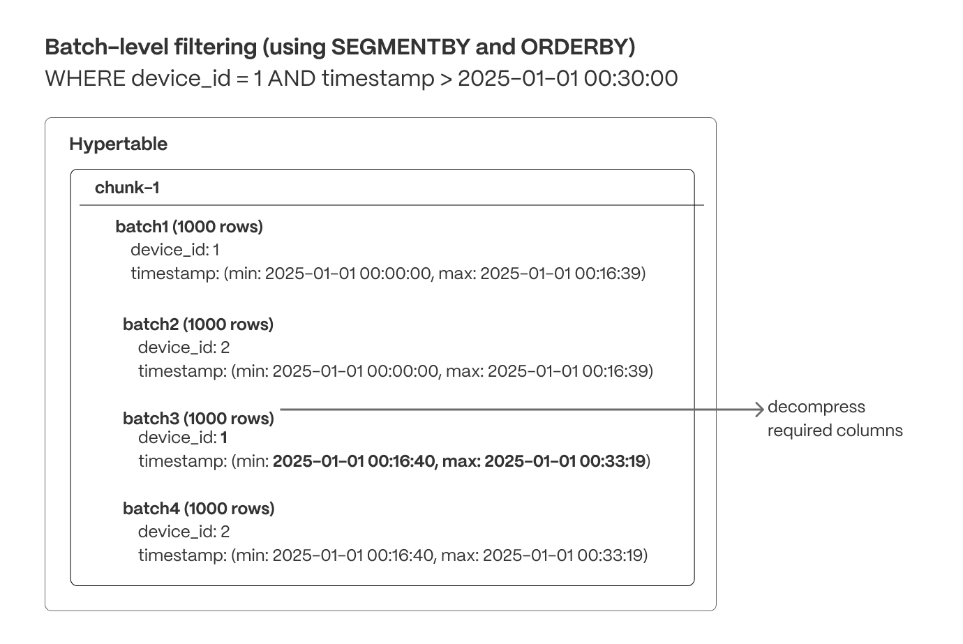
Batch-level filtering (columnar)

Within each chunk, compressed columnar batches are organized using SEGMENTBY keys and ordered by ORDERBY columns. Indexes and min/max metadata can be used to quickly exclude batches that don’t match the query criteria.

Maximize locality

Organizing data for efficient access ensures queries are read in the most optimal order, reducing unnecessary random reads and reducing scans of unneeded data.

Segmentation: Columnar batches are grouped using SEGMENTBY to keep related data together, improving scan efficiency.
Ordering: Data within each batch is physically sorted using ORDERBY, increasing scan efficiency (and reducing I/O operations), enabling efficient range queries, and minimizing post-query sorting.
Column selection: Queries read only the necessary columns, reducing disk I/O, decompression overhead, and memory usage.

Parallelize execution

Once a query is scanning only the required columnar data in the optimal order, TimescaleDB is able to maximize performance through parallel execution. As well as using multiple workers, TimescaleDB accelerates columnstore query execution by using Single Instruction, Multiple Data (SIMD) vectorization, allowing modern CPUs to process multiple data points in parallel.

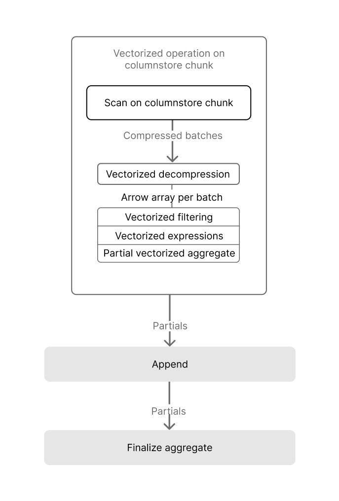
The TimescaleDB implementation of SIMD vectorization currently allows:

Vectorized decompression, which efficiently restores compressed data into a usable form for analysis.
Vectorized filtering, which rapidly applies filter conditions across data sets.
Vectorized aggregation, which performs aggregate calculations, such as sum or average, across multiple data points concurrently.

Accelerating queries with continuous aggregates

Aggregating large datasets in real time can be expensive, requiring repeated scans and calculations that strain CPU and I/O. While some databases attempt to brute-force these queries at runtime, compute and I/O are always finite resources—leading to high latency, unpredictable performance, and growing infrastructure costs as data volume increases.

Continuous aggregates, the TimescaleDB implementation of incrementally updated materialized views, solve this by shifting computation from every query run to a single, asynchronous step after data is ingested. Only the time buckets that receive new or modified data are updated, and queries read precomputed results instead of scanning raw data—dramatically improving performance and efficiency.

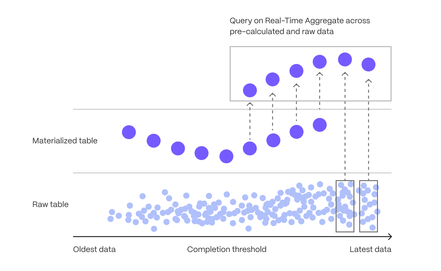
When you know the types of queries you'll need ahead of time, continuous aggregates allow you to pre-aggregate data along meaningful time intervals—such as per-minute, hourly, or daily summaries—delivering instant results without on-the-fly computation.

Continuous aggregates also avoid the time-consuming and error-prone process of maintaining manual rollups, while continuing to offer data mutability to support efficient updates, corrections, and backfills. Whenever new data is inserted or modified in chunks which have been materialized, TimescaleDB stores invalidation records reflecting that these results are stale and need to be recomputed. Then, an asynchronous process re-computes regions that include invalidated data, and updates the materialized results. TimescaleDB tracks the lineage and dependencies between continuous aggregates and their underlying data, to ensure the continuous aggregates are regularly kept up-to-date. This happens in a resource-efficient manner, and where multiple invalidations can be coalesced into a single refresh (as opposed to refreshing any dependencies at write time, such as via a trigger-based approach).

Continuous aggregates themselves are stored in hypertables, and they can be converted to columnar storage for compression, and raw data can be dropped, reducing storage footprint and processing cost. Continuous aggregates also support hierarchical rollups (e.g., hourly to daily to monthly) and real-time mode, which merges precomputed results with the latest ingested data to ensure accurate, up-to-date analytics.

This architecture enables scalable, low-latency analytics while keeping resource usage predictable—ideal for dashboards, monitoring systems, and any workload with known query patterns.

Hyperfunctions for real-time analytics

Real-time analytics requires more than basic SQL functions—efficient computation is essential as datasets grow in size and complexity. Hyperfunctions, available through the timescaledb_toolkit extension, provide high-performance, SQL-native functions tailored for time-series analysis. These include advanced tools for gap-filling, percentile estimation, time-weighted averages, counter correction, and state tracking, among others.

A key innovation of hyperfunctions is their support for partial aggregation, which allows TimescaleDB to store intermediate computational states rather than just final results. These partials can later be merged to compute rollups efficiently, avoiding expensive reprocessing of raw data and reducing compute overhead. This is especially effective when combined with continuous aggregates.

Consider a real-world example: monitoring request latencies across thousands of application instances. You might want to compute p95 latency per minute, then roll that up into hourly and daily percentiles for dashboards or alerts. With traditional SQL, calculating percentiles requires a full scan and sort of all underlying data—making multi-level rollups computationally expensive.

With TimescaleDB, you can use the percentile_agg hyperfunction in a continuous aggregate to compute and store a partial aggregation state for each minute. This state efficiently summarizes the distribution of latencies for that time bucket, without storing or sorting all individual values. Later, to produce an hourly or daily percentile, you simply combine the stored partials—no need to reprocess the raw latency values.

This approach provides a scalable, efficient solution for percentile-based analytics. By combining hyperfunctions with continuous aggregates, TimescaleDB enables real-time systems to deliver fast, resource-efficient insights across high-ingest, high-resolution datasets—without sacrificing accuracy or flexibility.

Cloud-native architecture

Real-time analytics requires a scalable, high-performance, and cost-efficient database that can handle high-ingest rates and low-latency queries without overprovisioning. Tiger Cloud is designed for elasticity, enabling independent scaling of storage and compute, workload isolation, and intelligent data tiering.

Independent storage and compute scaling

Real-time applications generate continuous data streams while requiring instant querying of both fresh and historical data. Traditional databases force users to pre-provision fixed storage, leading to unnecessary costs or unexpected limits. Tiger Cloud eliminates this constraint by dynamically scaling storage based on actual usage:

Storage expands and contracts automatically as data is added or deleted, avoiding manual intervention.
Usage-based billing ensures costs align with actual storage consumption, eliminating large upfront allocations.
Compute can be scaled independently to optimize query execution, ensuring fast analytics across both recent and historical data.

With this architecture, databases grow alongside data streams, enabling seamless access to real-time and historical insights while efficiently managing storage costs.

Workload isolation for real-time performance

Balancing high-ingest rates and low-latency analytical queries on the same system can create contention, slowing down performance. Tiger Cloud mitigates this by allowing read and write workloads to scale independently:

The primary database efficiently handles both ingestion and real-time rollups without disruption.
Read replicas scale query performance separately, ensuring fast analytics even under heavy workloads.

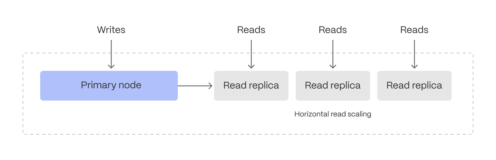
This separation ensures that frequent queries on fresh data don’t interfere with ingestion, making it easier to support live monitoring, anomaly detection, interactive dashboards, and alerting systems.

Intelligent data tiering for cost-efficient real-time analytics

Not all real-time data is equally valuable—recent data is queried constantly, while older data is accessed less frequently. Tiger Cloud can be configured to automatically tier data to cheaper bottomless object storage, ensuring that hot data remains instantly accessible, while historical data is still available.

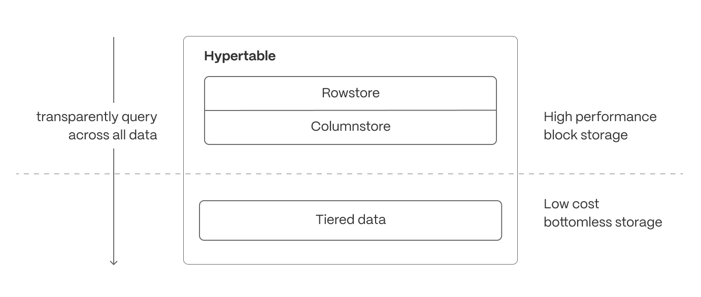
Recent, high-velocity data stays in high-performance storage for ultra-fast queries.
Older, less frequently accessed data is automatically moved to cost-efficient object storage but remains queryable and available for building continuous aggregates.

While many systems support this concept of data cooling, TimescaleDB ensures that the data can still be queried from the same hypertable regardless of its current location. For real-time analytics, this means applications can analyze live data streams without worrying about storage constraints, while still maintaining access to long-term trends when needed.

Cloud-native database observability

Real-time analytics doesn’t just require fast queries—it requires the ability to understand why queries are fast or slow, where resources are being used, and how performance changes over time. That’s why Tiger Cloud is built with deep observability features, giving developers and operators full visibility into their database workloads.

At the core of this observability is Insights, Tiger Cloud’s built-in query monitoring tool. Insights captures per-query statistics from our whole fleet in real time, showing you exactly how your database is behaving under load. It tracks key metrics like execution time, planning time, number of rows read and returned, I/O usage, and buffer cache hit rates—not just for the database as a whole, but for each individual query.

Insights lets you do the following:

Identify slow or resource-intensive queries instantly
Spot long-term performance regressions or trends
Understand query patterns and how they evolve over time
See the impact of schema changes, indexes, or continuous aggregates on workload performance
Monitor and compare different versions of the same query to optimize execution

All this is surfaced through an intuitive interface, available directly in Tiger Cloud, with no instrumentation or external monitoring infrastructure required.

Beyond query-level visibility, Tiger Cloud also exposes metrics around service resource consumption, compression, continuous aggregates, and data tiering, allowing you to track how data moves through the system—and how those background processes impact storage and query performance.

Together, these observability features give you the insight and control needed to operate a real-time analytics database at scale, with confidence, clarity, and performance you can trust.

Ensuring reliability and scalability

Maintaining high availability, efficient resource utilization, and data durability is essential for real-time applications. Tiger Cloud provides robust operational features to ensure seamless performance under varying workloads.

High-availability (HA) replicas: deploy multi-AZ HA replicas to provide fault tolerance and ensure minimal downtime. In the event of a primary node failure, replicas are automatically promoted to maintain service continuity.
Connection pooling: optimize database connections by efficiently managing and reusing them, reducing overhead and improving performance for high-concurrency applications.
Backup and recovery: leverage continuous backups, Point-in-Time Recovery (PITR), and automated snapshotting to protect against data loss. Restore data efficiently to minimize downtime in case of failures or accidental deletions.

These operational capabilities ensure Tiger Cloud remains reliable, scalable, and resilient, even under demanding real-time workloads.

Real-time analytics is critical for modern applications, but traditional databases struggle to balance high-ingest performance, low-latency queries, and flexible data mutability. Tiger Cloud extends Postgres to solve this challenge, combining automatic partitioning, hybrid row-columnar storage, and intelligent compression to optimize both transactional and analytical workloads.

With continuous aggregates, hyperfunctions, and advanced query optimizations, Tiger Cloud ensures sub-second queries even on massive datasets that combine current and historic data. Its cloud-native architecture further enhances scalability with independent compute and storage scaling, workload isolation, and cost-efficient data tiering—allowing applications to handle real-time and historical queries seamlessly.

For developers, this means building high-performance, real-time analytics applications without sacrificing SQL compatibility, transactional guarantees, or operational simplicity.

Tiger Cloud delivers the best of Postgres, optimized for real-time analytics.

===== PAGE: https://docs.tigerdata.com/about/pricing-and-account-management/ =====

stddev()

URL: llms-txt#stddev()

===== PAGE: https://docs.tigerdata.com/api/_hyperfunctions/stats_agg-one-variable/rollup/ =====

Approximate percentiles

URL: llms-txt#approximate-percentiles

Contents:

Run an approximate percentage query
- Running an approximate percentage query

TimescaleDB uses approximation algorithms to calculate a percentile without requiring all of the data. This also makes them more compatible with continuous aggregates.

By default, TimescaleDB Toolkit uses uddsketch, but you can also choose to use tdigest. For more information about these algorithms, see the [advanced aggregation methods][advanced-agg] documentation.

Run an approximate percentage query

In this procedure, we use an example table called response_times that contains information about how long a server takes to respond to API calls.

Running an approximate percentage query

At the psql prompt, create a continuous aggregate that computes the daily aggregates:
Re-aggregate the aggregate to get the last 30 days, and look for the ninety-fifth percentile:
You can also create an alert:

For more information about percentile approximation API calls, see the [hyperfunction API documentation][hyperfunctions-api-approx-percentile].

===== PAGE: https://docs.tigerdata.com/use-timescale/hyperfunctions/index/ =====

Examples:

Example 1 (sql):

CREATE MATERIALIZED VIEW response_times_daily
    WITH (timescaledb.continuous)
    AS SELECT
      time_bucket('1 day'::interval, ts) as bucket,
      percentile_agg(response_time_ms)
    FROM response_times
    GROUP BY 1;

Example 2 (sql):

SELECT approx_percentile(0.95, percentile_agg) as threshold
    FROM response_times_daily
    WHERE bucket >= time_bucket('1 day'::interval, now() - '30 days'::interval);

Example 3 (sql):

WITH t as (SELECT approx_percentile(0.95, percentile_agg(percentile_agg)) as threshold
    FROM response_times_daily
    WHERE bucket >= time_bucket('1 day'::interval, now() - '30 days'::interval))

    SELECT count(*)
    FROM response_times
    WHERE ts > now()- '1 minute'::interval
    AND response_time_ms > (SELECT threshold FROM t);

skewness_y() | skewness_x()

URL: llms-txt#skewness_y()-|-skewness_x()

===== PAGE: https://docs.tigerdata.com/api/_hyperfunctions/stats_agg-two-variables/num_vals/ =====

covariance()

URL: llms-txt#covariance()

===== PAGE: https://docs.tigerdata.com/api/_hyperfunctions/stats_agg-two-variables/rolling/ =====

hyperfunctions.md 79 KB Geçmiş Ham

Timescaledb - Hyperfunctions

stddev_y() | stddev_x()

timescaledb_information.job_stats

percentile_agg()

x_intercept()

approx_percentile_rank()

mean()

Hyperfunctions

Learn hyperfunction basics and install TimescaleDB Toolkit

Browse hyperfunctions and TimescaleDB Toolkit features by category

Troubleshooting hyperfunctions and TimescaleDB Toolkit

Updating the Toolkit extension fails with an error saying no update path

Troubleshooting Toolkit setup

Analytics on transport and geospatial data

Optimize time-series data in hypertables

Optimize your data for real-time analytics

Connect Grafana to Tiger Cloud

Monitor performance over time

Optimize revenue potential

Set up your data for geospatial queries

Visualize the area where you can make the most money

variance_y() | variance_x()

approx_percentile()

sum()

sum_y() | sum_x()

About TimescaleDB hyperfunctions

Available hyperfunctions

Function pipelines

Toolkit feature development

Contribute to TimescaleDB Toolkit

kurtosis()

num_vals()

Last observation carried forward

kurtosis_y() | kurtosis_x()

average_y() | average_x()

Real-time analytics with Tiger Cloud and Grafana

Optimize time-series data in hypertables

Optimize your data for real-time analytics

Write fast analytical queries

Connect Grafana to Tiger Cloud

Visualize energy consumption

stats_agg() (one variable)

rollup()

Percentile approximation

stats_agg() (two variables)

skewness()

rolling()

uddsketch()

determination_coeff()

approx_percentile_array()

Tiger Data architecture for real-time analytics

What is real-time analytics?

Tiger Cloud: real-time analytics from Postgres

Efficient data partitioning

Row-columnar storage

Columnar storage layout

Columnar batches

Segmenting and ordering data

Real-time writes without delays

Efficient updates and deletes without performance penalties

Query optimizations

Skip unnecessary data

Primary partition exclusion (row and columnar)

Secondary partition exclusion (columnar)

Postgres indexes (row and columnar)

Batch-level filtering (columnar)

Maximize locality

Parallelize execution

Accelerating queries with continuous aggregates

Hyperfunctions for real-time analytics

Cloud-native architecture

Independent storage and compute scaling

Workload isolation for real-time performance

Intelligent data tiering for cost-efficient real-time analytics

Cloud-native database observability

Ensuring reliability and scalability

stddev()

Approximate percentiles

Run an approximate percentage query

hyperfunctions.md 79 KB

Geçmiş Ham

Updating the Toolkit extension fails with an error saying `no update path`