
time_buckets.md 53 KB
Timescaledb - Time Buckets
Pages: 16
Gapfilling and interpolation
URL: llms-txt#gapfilling-and-interpolation
Most time-series data analysis techniques aggregate data into fixed time intervals, which smooths the data and makes it easier to interpret and analyze. When you write queries for data in this form, you need an efficient way to aggregate raw observations, which are often noisy and irregular, in to fixed time intervals. TimescaleDB does this using time bucketing, which gives a clear picture of the important data trends using a concise, declarative SQL query.
Sorting data into time buckets works well in most cases, but problems can arise if there are gaps in the data. This can happen if you have irregular sampling intervals, or you have experienced an outage of some sort. You can use a gapfilling function to create additional rows of data in any gaps, ensuring that the returned rows are in chronological order, and contiguous.
- For more information about how gapfilling works, read our [gapfilling blog][blog-gapfilling].
- For more information about gapfilling and interpolation API calls, see the [hyperfunction API documentation][hyperfunctions-api-gapfilling].
===== PAGE: https://docs.tigerdata.com/use-timescale/hyperfunctions/approximate-percentile/ =====
time_bucket_gapfill()
URL: llms-txt#time_bucket_gapfill()
===== PAGE: https://docs.tigerdata.com/api/_hyperfunctions/time_bucket_gapfill/intro/ =====
Aggregate data by time interval, while filling in gaps of missing data.
time_bucket_gapfill works similarly to [time_bucket][time_bucket], but adds
gapfilling capabilities. The other functions in this group must be used in the
same query as time_bucket_gapfill. They control how missing values are treated.
time_bucket_gapfill must be used as a top-level expression in a query or
subquery. You cannot, for example, nest time_bucket_gapfill in another
function (such as round(time_bucket_gapfill(...))), or cast the result of the
gapfilling call. If you need to cast, you can use time_bucket_gapfill in a
subquery, and let the outer query do the type cast.
===== PAGE: https://docs.tigerdata.com/api/_hyperfunctions/time_bucket_gapfill/locf/ =====
State aggregates
URL: llms-txt#state-aggregates
Contents:
- Notes on compact_state_agg and state_agg
- Hyperfunctions
This section includes functions used to measure the time spent in a relatively small number of states.
For these hyperfunctions, you need to install the [TimescaleDB Toolkit][install-toolkit] Postgres extension.
Notes on compact_state_agg and state_agg
state_agg supports all hyperfunctions that operate on CompactStateAggs, in addition
to some additional functions that need a full state timeline.
All compact_state_agg and state_agg hyperfunctions support both string (TEXT) and integer (BIGINT) states.
You can't mix different types of states within a single aggregate.
Integer states are useful when the state value is a foreign key representing a row in another table that stores all possible states.
<HyperfunctionTable
hyperfunctionFamily='state aggregates'
includeExperimental
sortByType
/>
===== PAGE: https://docs.tigerdata.com/api/index/ =====
timescaledb_information.continuous_aggregates
URL: llms-txt#timescaledb_information.continuous_aggregates
Contents:
- Samples
- Available columns
Get metadata and settings information for continuous aggregates.
| Name | Type | Description |
|---|---|---|
hypertable_schema |
TEXT | Schema of the hypertable from the continuous aggregate view |
hypertable_name |
TEXT | Name of the hypertable from the continuous aggregate view |
view_schema |
TEXT | Schema for continuous aggregate view |
view_name |
TEXT | User supplied name for continuous aggregate view |
view_owner |
TEXT | Owner of the continuous aggregate view |
materialized_only |
BOOLEAN | Return only materialized data when querying the continuous aggregate view |
compression_enabled |
BOOLEAN | Is compression enabled for the continuous aggregate view? |
materialization_hypertable_schema |
TEXT | Schema of the underlying materialization table |
materialization_hypertable_name |
TEXT | Name of the underlying materialization table |
view_definition |
TEXT | SELECT query for continuous aggregate view |
finalized |
BOOLEAN | Whether the continuous aggregate stores data in finalized or partial form. Since TimescaleDB 2.7, the default is finalized. |
===== PAGE: https://docs.tigerdata.com/api/jobs-automation/alter_job/ =====
Examples:
Example 1 (sql):
SELECT * FROM timescaledb_information.continuous_aggregates;

-[ RECORD 1 ]---------------------+-------------------------------------------------
hypertable_schema                 | public
hypertable_name                   | foo
view_schema                       | public
view_name                         | contagg_view
view_owner                        | postgres
materialized_only                 | f
compression_enabled               | f
materialization_hypertable_schema | _timescaledb_internal
materialization_hypertable_name   | _materialized_hypertable_2
view_definition                   |  SELECT foo.a,                                  +
                                  |     COUNT(foo.b) AS countb                      +
                                  |    FROM foo                                     +
                                  |   GROUP BY (time_bucket('1 day', foo.a)), foo.a;
finalized                         | t
timescaledb_experimental.time_bucket_ng()
URL: llms-txt#timescaledb_experimental.time_bucket_ng()
Contents:
- Samples
- Required arguments
- Optional arguments
- Returns
The time_bucket_ng() function is an experimental version of the
[time_bucket()][time_bucket] function. It introduced some new capabilities,
such as monthly buckets and timezone support. Those features are now part of the
regular time_bucket() function.
This section describes a feature that is deprecated. We strongly recommend that you do not use this feature in a production environment. If you need more information, contact us.
The time_bucket() and time_bucket_ng() functions are similar, but not
completely compatible. There are two main differences.
Firstly, time_bucket_ng() doesn't work with timestamps prior to origin,
while time_bucket() does.
Secondly, the default origin values differ. time_bucket() uses an origin
date of January 3, 2000, for buckets shorter than a month. time_bucket_ng()
uses an origin date of January 1, 2000, for all bucket sizes.
In this example, time_bucket_ng() is used to create bucket data in three month
intervals:
This example uses time_bucket_ng() to bucket data in one year intervals:
To split time into buckets, time_bucket_ng() uses a starting point in time
called origin. The default origin is 2000-01-01. time_bucket_ng cannot use
timestamps earlier than origin:
Going back in time from origin isn't usually possible, especially when you
consider timezones and daylight savings time (DST). Note also that there is no
reasonable way to split time in variable-sized buckets (such as months) from an
arbitrary origin, so origin defaults to the first day of the month.
To bypass named limitations, you can override the default origin:
This example shows how time_bucket_ng() is used to bucket data
by months in a specified timezone:
You can use time_bucket_ng() with continuous aggregates. This example tracks
the temperature in Moscow over seven day intervals:
The by_range dimension builder is an addition to TimescaleDB
2.13. For simpler cases, like this one, you can also create the
hypertable using the old syntax:
For more information, see the [continuous aggregates documentation][caggs].
While time_bucket_ng() supports months and timezones,
continuous aggregates cannot always be used with monthly
buckets or buckets with timezones.
This table shows which time_bucket_ng() functions can be used in a continuous aggregate:
|Function|Available in continuous aggregate|TimescaleDB version| |-|-|-| |Buckets by seconds, minutes, hours, days, and weeks|✅|2.4.0 - 2.14.2| |Buckets by months and years|✅|2.6.0 - 2.14.2| |Timezones support|✅|2.6.0 - 2.14.2| |Specify custom origin|✅|2.7.0 - 2.14.2|
Required arguments
| Name | Type | Description |
|---|---|---|
bucket_width |
INTERVAL | A Postgres time interval for how long each bucket is |
ts |
DATE, TIMESTAMP or TIMESTAMPTZ | The timestamp to bucket |
Optional arguments
| Name | Type | Description |
|---|---|---|
origin |
Should be the same as ts |
Buckets are aligned relative to this timestamp |
timezone |
TEXT | The name of the timezone. The argument can be specified only if the type of ts is TIMESTAMPTZ |
For backward compatibility with time_bucket() the timezone argument is
optional. However, it is required for time buckets that are less than 24 hours.
If you call the TIMESTAMPTZ-version of the function without the timezone
argument, the timezone defaults to the session's timezone and so the function
can't be used with continuous aggregates. Best practice is to use
time_bucket_ng(interval, timestamptz, text) and specify the timezone.
The function returns the bucket's start time. The return value type is the
same as ts.
===== PAGE: https://docs.tigerdata.com/api/days_in_month/ =====
Examples:
Example 1 (sql):
SELECT timescaledb_experimental.time_bucket_ng('3 month', date '2021-08-01');
 time_bucket_ng
----------------
 2021-07-01
(1 row)
Example 2 (sql):
SELECT timescaledb_experimental.time_bucket_ng('1 year', date '2021-08-01');
 time_bucket_ng
----------------
 2021-01-01
(1 row)
Example 3 (sql):
SELECT timescaledb_experimental.time_bucket_ng('100 years', timestamp '1988-05-08');
ERROR:  origin must be before the given date
Example 4 (sql):
-- working with timestamps before 2000-01-01
SELECT timescaledb_experimental.time_bucket_ng('100 years', timestamp '1988-05-08', origin => '1900-01-01');
   time_bucket_ng
---------------------
 1900-01-01 00:00:00

-- unlike the default origin, which is Saturday, 2000-01-03 is Monday
SELECT timescaledb_experimental.time_bucket_ng('1 week', timestamp '2021-08-26', origin => '2000-01-03');
   time_bucket_ng
---------------------
 2021-08-23 00:00:00
add_continuous_aggregate_policy()
URL: llms-txt#add_continuous_aggregate_policy()
Contents:
- Samples
- Required arguments
- Optional arguments
- Returns
Create a policy that automatically refreshes a continuous aggregate. To view the policies that you set or the policies that already exist, see [informational views][informational-views].
Add a policy that refreshes the last month once an hour, excluding the latest hour from the aggregate. For performance reasons, we recommend that you exclude buckets that see lots of writes:
Required arguments
|Name|Type|Description|
|-|-|-|
|continuous_aggregate|REGCLASS|The continuous aggregate to add the policy for|
|start_offset|INTERVAL or integer|Start of the refresh window as an interval relative to the time when the policy is executed. NULL is equivalent to MIN(timestamp) of the hypertable.|
|end_offset|INTERVAL or integer|End of the refresh window as an interval relative to the time when the policy is executed. NULL is equivalent to MAX(timestamp) of the hypertable.|
|schedule_interval|INTERVAL|Interval between refresh executions in wall-clock time. Defaults to 24 hours|
|initial_start|TIMESTAMPTZ|Time the policy is first run. Defaults to NULL. If omitted, then the schedule interval is the intervalbetween the finish time of the last execution and the next start. If provided, it serves as the origin with respect to which the next_start is calculated |
The start_offset should be greater than end_offset.
You must specify the start_offset and end_offset parameters differently,
depending on the type of the time column of the hypertable:
- For hypertables with
TIMESTAMP,TIMESTAMPTZ, andDATEtime columns, set the offset as anINTERVALtype. - For hypertables with integer-based timestamps, set the offset as an
INTEGERtype.
While setting end_offset to NULL is possible, it is not recommended. To include the data between end_offset and
the current time in queries, enable real-time aggregation.
You can add concurrent refresh policies on each continuous aggregate, as long as the start_offset and end_offset does not overlap with another policy on the same continuous aggregate.
Optional arguments
|Name|Type|Description|
|-|-|-|
|if_not_exists|BOOLEAN|Set to true to issue a notice instead of an error if the job already exists. Defaults to false.|
|timezone|TEXT|A valid time zone. If you specify initial_start, subsequent executions of the refresh policy are aligned on initial_start. However, daylight savings time (DST) changes may shift this alignment. If this is an issue you want to mitigate, set timezone to a valid time zone. Default is NULL, UTC bucketing is performed.|
| include_tiered_data | BOOLEAN | Enable/disable reading tiered data. This setting helps override the current settings for thetimescaledb.enable_tiered_reads GUC. The default is NULL i.e we use the current setting for timescaledb.enable_tiered_reads GUC | |
| buckets_per_batch | INTEGER | Number of buckets to be refreshed by a batch. This value is multiplied by the CAgg bucket width to determine the size of the batch range. Default value is 1, single batch execution. Values of less than 0 are not allowed. | |
| max_batches_per_execution | INTEGER | Limit the maximum number of batches to run when a policy executes. If some batches remain, they are processed the next time the policy runs. Default value is 0, for an unlimted number of batches. Values of less than 0 are not allowed. | |
| refresh_newest_first | BOOLEAN | Control the order of incremental refreshes. Set to TRUE to refresh from the newest data to the oldest. Set to FALSE for oldest to newest. The default is TRUE. | |
Setting buckets_per_batch greater than zero means that the refresh window is split in batches of bucket width * buckets per batch. For example, a given Continuous Aggregate with bucket width of 1 day and buckets_per_batch of 10 has a batch size of 10 days to process the refresh.
Because each batch is an individual transaction, executing a policy in batches make the data visible for the users before the entire job is executed. Batches are processed from the most recent data to the oldest.
|Column|Type|Description|
|-|-|-|
|job_id|INTEGER|TimescaleDB background job ID created to implement this policy|
===== PAGE: https://docs.tigerdata.com/api/continuous-aggregates/hypertable_size/ =====
Examples:
Example 1 (sql):
SELECT add_continuous_aggregate_policy('conditions_summary',
  start_offset => INTERVAL '1 month',
  end_offset => INTERVAL '1 hour',
  schedule_interval => INTERVAL '1 hour');
remove_continuous_aggregate_policy()
URL: llms-txt#remove_continuous_aggregate_policy()
Contents:
- Samples
- Required arguments
- Optional arguments
Remove all refresh policies from a continuous aggregate.
To view the existing continuous aggregate policies, see the policies informational view.
Remove all refresh policies from the cpu_view continuous aggregate:
Required arguments
|Name|Type|Description|
|-|-|-|
|continuous_aggregate|REGCLASS|Name of the continuous aggregate the policies should be removed from|
Optional arguments
|Name|Type|Description|
|-|-|-|
|if_exists (formerly if_not_exists)|BOOL|When true, prints a warning instead of erroring if the policy doesn't exist. Defaults to false. Renamed in TimescaleDB 2.8.|
===== PAGE: https://docs.tigerdata.com/api/continuous-aggregates/add_policies/ =====
Examples:
Example 1 (sql):
remove_continuous_aggregate_policy(
    continuous_aggregate REGCLASS,
    if_exists BOOL = NULL
) RETURNS VOID
Percentile approximation advanced aggregation methods
URL: llms-txt#percentile-approximation-advanced-aggregation-methods
Contents:
- Choose the right algorithm
TimescaleDB uses approximation algorithms to calculate a percentile without
requiring all of the data. This also makes them more compatible with continuous
aggregates. By default, TimescaleDB uses uddsketch, but you can also choose to
use tdigest. This section describes the different methods, and helps you to
decide which one you should use.
uddsketch is the default algorithm. It uses exponentially sized buckets to
guarantee the approximation falls within a known error range, relative to the
true discrete percentile. This algorithm offers the ability to tune the size and
maximum error target of the sketch.
tdigest buckets data more aggressively toward the center of the quantile
range, giving it greater accuracy at the tails of the range, around 0.001 or
0.995.
Choose the right algorithm
Each algorithm has different features, which can make one better than another depending on your use case. Here are some of the differences to consider when choosing an algorithm:
Before you begin, it is important to understand that the formal definition for
a percentile is imprecise, and there are different methods for determining what
the true percentile actually is. In Postgres, given a target percentile p,
[percentile_disc][pg-percentile] returns the smallest element of a set, so
that p percent of the set is less than that element. However,
[percentile_cont][pg-percentile] returns an interpolated value between the two
nearest matches for p. In practice, the difference between these methods is
very small but, if it matters to your use case, keep in mind that tdigest
approximates the continuous percentile, while uddsketch provides an estimate
of the discrete value.
Think about the types of percentiles you're most interested in. tdigest is
optimized for more accurate estimates at the extremes, and less accurate
estimates near the median. If your workflow involves estimating ninety-ninth
percentiles, then choose tdigest. If you're more concerned about getting
highly accurate median estimates, choose uddsketch.
The algorithms differ in the way they estimate data. uddsketch has a stable
bucketing function, so it always returns the same percentile estimate for
the same underlying data, regardless of how it is ordered or re-aggregated. On
the other hand, tdigest builds up incremental buckets based on the average of
nearby points, which can result in some subtle differences in estimates based on
the same data unless the order and batching of the aggregation is strictly
controlled, which is sometimes difficult to do in Postgres. If stable
estimates are important to you, choose uddsketch.
Calculating precise error bars for tdigest can be difficult, especially when
merging multiple sub-digests into a larger one. This can occur through summary
aggregation, or parallelization of the normal point aggregate. If you need to
tightly characterize your errors, choose uddsketch. However, because
uddsketch uses exponential bucketing to provide a guaranteed relative error,
it can cause some wildly varying absolute errors if the dataset covers a large
range. For example, if the data is evenly distributed over the range [1,100],
estimates at the high end of the percentile range have about 100 times the
absolute error of those at the low end of the range. This gets much more extreme
if the data range is [0,100]. If having a stable absolute error is important to
your use case, choose tdigest.
While both algorithms are likely to get smaller and faster with future
optimizations, uddsketch generally requires a smaller memory footprint than
tdigest, and a correspondingly smaller disk footprint for any continuous
aggregates. Regardless of the algorithm you choose, the best way to improve the
accuracy of your percentile estimates is to increase the number of buckets,
which is simpler to do with uddsketch. If your use case does not get a clear
benefit from using tdigest, the default uddsketch is your best choice.
For some more technical details and usage examples of the different algorithms, see the developer documentation for [uddsketch][gh-uddsketch] and [tdigest][gh-tdigest].
===== PAGE: https://docs.tigerdata.com/use-timescale/hyperfunctions/locf/ =====
state_periods()
URL: llms-txt#state_periods()
===== PAGE: https://docs.tigerdata.com/api/_hyperfunctions/time_bucket_gapfill/interpolate/ =====
time_bucket()
URL: llms-txt#time_bucket()
Contents:
- Samples
- Required arguments for interval time inputs
- Optional arguments for interval time inputs
- Required arguments for integer time inputs
- Optional arguments for integer time inputs
The time_bucket function is similar to the standard Postgres date_bin
function. Unlike date_bin, it allows for arbitrary time intervals of months or
longer. The return value is the bucket's start time.
Buckets are aligned to start at midnight in UTC+0. The time bucket size (bucket_width) can be set as INTERVAL or INTEGER. For INTERVAL-type bucket_width, you can change the time zone with the optional timezone parameter. In this case, the buckets are realigned to start at midnight in the time zone you specify.
Note that during shifts to and from daylight savings, the amount of data
aggregated into the corresponding buckets can be irregular. For example, if the
bucket_width is 2 hours, the number of bucketed hours is either three hours or one hour.
Simple five-minute averaging:
To report the middle of the bucket, instead of the left edge:
For rounding, move the alignment so that the middle of the bucket is at the five-minute mark, and report the middle of the bucket:
In this example, add the explicit cast to ensure that Postgres chooses the correct function.
To shift the alignment of the buckets, you can use the origin parameter passed as a timestamp, timestamptz, or date type. This example shifts the start of the week to a Sunday, instead of the default of Monday:
The value of the origin parameter in this example is 2017-12-31, a Sunday
within the period being analyzed. However, the origin provided to the function
can be before, during, or after the data being analyzed. All buckets are
calculated relative to this origin. So, in this example, any Sunday could have
been used. Note that because time < TIMESTAMPTZ '2018-01-03' is used in this
example, the last bucket would have only 4 days of data. This cast to TIMESTAMP
converts the time to local time according to the server's time zone setting.
Bucket temperature values to calculate the average monthly temperature. Set the time zone to 'Europe/Berlin' so bucket start and end times are aligned to midnight in Berlin.
Required arguments for interval time inputs
|Name|Type|Description|
|-|-|-|
|bucket_width|INTERVAL|A Postgres time interval for how long each bucket is|
|ts|DATE, TIMESTAMP, or TIMESTAMPTZ|The timestamp to bucket|
If you use months as an interval for bucket_width, you cannot combine it with
a non-month component. For example, 1 month and 3 months are both valid
bucket widths, but 1 month 1 day and 3 months 2 weeks are not.
Optional arguments for interval time inputs
|Name|Type| Description |
|-|-|------------------------------------------------------------------------------------------------------------------------------------------------------------------------------------------------------------------------------------------------------------------------------------------------|
|timezone|TEXT| The time zone for calculating bucket start and end times. Can only be used with TIMESTAMPTZ. Defaults to UTC+0. |
|origin|DATE, TIMESTAMP, or TIMESTAMPTZ| Buckets are aligned relative to this timestamp. Defaults to midnight on January 3, 2000, for buckets that don't include a month or year interval, and to midnight on January 1, 2000, for month, year, and century buckets. |
|offset|INTERVAL| The time interval to offset all time buckets by. A positive value shifts bucket start and end times later. A negative value shifts bucket start and end times earlier. offset must be surrounded with double quotes when used as a named argument, because it is a reserved key word in Postgres. |
Required arguments for integer time inputs
|Name|Type|Description|
|-|-|-|
|bucket_width|INTEGER|The bucket width|
|ts|INTEGER|The timestamp to bucket|
Optional arguments for integer time inputs
|Name|Type|Description|
|-|-|-|
|offset|INTEGER|The amount to offset all buckets by. A positive value shifts bucket start and end times later. A negative value shifts bucket start and end times earlier. offset must be surrounded with double quotes when used as a named argument, because it is a reserved key word in Postgres.|
===== PAGE: https://docs.tigerdata.com/api/time_bucket_ng/ =====
Examples:
Example 1 (sql):
SELECT time_bucket('5 minutes', time) AS five_min, avg(cpu)
FROM metrics
GROUP BY five_min
ORDER BY five_min DESC LIMIT 10;
Example 2 (sql):
SELECT time_bucket('5 minutes', time) + '2.5 minutes'
  AS five_min, avg(cpu)
FROM metrics
GROUP BY five_min
ORDER BY five_min DESC LIMIT 10;
Example 3 (sql):
SELECT time_bucket('5 minutes', time, '-2.5 minutes'::INTERVAL) + '2.5 minutes'
  AS five_min, avg(cpu)
FROM metrics
GROUP BY five_min
ORDER BY five_min DESC LIMIT 10;
Example 4 (sql):
SELECT time_bucket('1 week', timetz, TIMESTAMPTZ '2017-12-31')
  AS one_week, avg(cpu)
FROM metrics
GROUP BY one_week
WHERE time > TIMESTAMPTZ '2017-12-01'  AND time < TIMESTAMPTZ '2018-01-03'
ORDER BY one_week DESC LIMIT 10;
Query data
URL: llms-txt#query-data
Hypertables in TimescaleDB are Postgres tables. That means you can query them with standard SQL commands.
- [About querying data][about-querying-data]
- [Select data with
SELECT][selecting-data] - [Get faster
DISTINCTqueries with SkipScan][skipscan] - [Perform advanced analytic queries][advanced-analytics]
===== PAGE: https://docs.tigerdata.com/use-timescale/time-buckets/ =====
Analyze financial tick data - Query the data
URL: llms-txt#analyze-financial-tick-data---query-the-data
Contents:
- Create a continuous aggregate
- Creating a continuous aggregate
- Query the continuous aggregate
- Querying the continuous aggregate
- Graph OHLCV data
- Graphing OHLCV data
Turning raw, real-time tick data into aggregated candlestick views is a common task for users who work with financial data. TimescaleDB includes [hyperfunctions][hyperfunctions] that you can use to store and query your financial data more easily. Hyperfunctions are SQL functions within TimescaleDB that make it easier to manipulate and analyze time-series data in Postgres with fewer lines of code.
There are three hyperfunctions that are essential for calculating candlestick
values: [time_bucket()][time-bucket], [FIRST()][first], and [LAST()][last].
The time_bucket() hyperfunction helps you aggregate records into buckets of
arbitrary time intervals based on the timestamp value. FIRST() and LAST()
help you calculate the opening and closing prices. To calculate highest and
lowest prices, you can use the standard Postgres aggregate functions MIN and
MAX.
In TimescaleDB, the most efficient way to create candlestick views is to use [continuous aggregates][caggs]. In this tutorial, you create a continuous aggregate for a candlestick time bucket, and then query the aggregate with different refresh policies. Finally, you can use Grafana to visualize your data as a candlestick chart.
Create a continuous aggregate
To look at OHLCV values, the most effective way is to create a continuous aggregate. In this tutorial, you create a continuous aggregate to aggregate data for each day. You then set the aggregate to refresh every day, and to aggregate the last two days' worth of data.
Creating a continuous aggregate
Connect to the Tiger Cloud service that contains the Twelve Data cryptocurrency dataset.
At the psql prompt, create the continuous aggregate to aggregate data every minute:
When you create the continuous aggregate, it refreshes by default.
- Set a refresh policy to update the continuous aggregate every day, if there is new data available in the hypertable for the last two days:
Query the continuous aggregate
When you have your continuous aggregate set up, you can query it to get the OHLCV values.
Querying the continuous aggregate
Connect to the Tiger Cloud service that contains the Twelve Data cryptocurrency dataset.
At the psql prompt, use this query to select all Bitcoin OHLCV data for the past 14 days, by time bucket:
The result of the query looks like this:
When you have extracted the raw OHLCV data, you can use it to graph the result in a candlestick chart, using Grafana. To do this, you need to have Grafana set up to connect to your self-hosted TimescaleDB instance.
Graphing OHLCV data
- Ensure you have Grafana installed, and you are using the TimescaleDB database that contains the Twelve Data dataset set up as a data source.
- In Grafana, from the
Dashboardsmenu, clickNew Dashboard. In theNew Dashboardpage, clickAdd a new panel. - In the
Visualizationsmenu in the top right corner, selectCandlestickfrom the list. Ensure you have set the Twelve Data dataset as your data source. - Click
Edit SQLand paste in the query you used to get the OHLCV values. - In the
Format assection, selectTable. - Adjust elements of the table as required, and click
Applyto save your graph to the dashboard.
<img class="main-content__illustration"
     width={1375} height={944}
     src="https://assets.timescale.com/docs/images/Grafana_candlestick_1day.webp"
     alt="Creating a candlestick graph in Grafana using 1-day OHLCV tick data"
/>
===== PAGE: https://docs.tigerdata.com/tutorials/blockchain-analyze/blockchain-dataset/ =====
Examples:
Example 1 (sql):
CREATE MATERIALIZED VIEW one_day_candle
    WITH (timescaledb.continuous) AS
        SELECT
            time_bucket('1 day', time) AS bucket,
            symbol,
            FIRST(price, time) AS "open",
            MAX(price) AS high,
            MIN(price) AS low,
            LAST(price, time) AS "close",
            LAST(day_volume, time) AS day_volume
        FROM crypto_ticks
        GROUP BY bucket, symbol;
Example 2 (sql):
SELECT add_continuous_aggregate_policy('one_day_candle',
        start_offset => INTERVAL '3 days',
        end_offset => INTERVAL '1 day',
        schedule_interval => INTERVAL '1 day');
Example 3 (sql):
SELECT * FROM one_day_candle
    WHERE symbol = 'BTC/USD' AND bucket >= NOW() - INTERVAL '14 days'
    ORDER BY bucket;
Example 4 (sql):
bucket         | symbol  |  open   |  high   |   low   |  close  | day_volume
    ------------------------+---------+---------+---------+---------+---------+------------
     2022-11-24 00:00:00+00 | BTC/USD |   16587 | 16781.2 | 16463.4 | 16597.4 |      21803
     2022-11-25 00:00:00+00 | BTC/USD | 16597.4 | 16610.1 | 16344.4 | 16503.1 |      20788
     2022-11-26 00:00:00+00 | BTC/USD | 16507.9 | 16685.5 | 16384.5 | 16450.6 |      12300
Updates to previously materialized regions aren't shown in real-time aggregates
URL: llms-txt#updates-to-previously-materialized-regions-aren't-shown-in-real-time-aggregates
Real-time aggregates automatically add the most recent data when you query your continuous aggregate. In other words, they include data more recent than your last materialized bucket.
If you add new historical data to an already-materialized bucket, it won't be
reflected in a real-time aggregate. You should wait for the next scheduled
refresh, or manually refresh by calling refresh_continuous_aggregate. You can
think of real-time aggregates as being eventually consistent for historical
data.
The following example shows how this works:
- Create the hypertable:
If you are self-hosting TimescaleDB v2.19.3 and below, create a [Postgres relational table][pg-create-table], then convert it using [create_hypertable][create_hypertable]. You then enable hypercore with a call to [ALTER TABLE][alter_table_hypercore].
Add data to your hypertable:
Create a continuous aggregate but do not materialize any data:
Create the continuous aggregate:
Check your data:
The query on the continuous aggregate fetches data directly from the hypertable:
| city | bucket | min | max|
  |--------|------------|-----|-----|
  | Moscow | 2021-06-14 |  22 |  30 |
  | Moscow | 2021-06-21 |  31 |  34 |
Materialize data into the continuous aggregate:
Add a refresh policy:
Check your data:
The select query returns the same data, as expected, but this time the data is fetched from the underlying materialized table
| city | bucket | min | max|
  |--------|------------|-----|-----|
  | Moscow | 2021-06-14 |  22 |  30 |
  | Moscow | 2021-06-21 |  31 |  34 |
Update the data in the previously materialized bucket:
Update the data in your hypertable:
Check your data:
The updated data is not yet visible when you query the continuous aggregate. This is because these changes have not been materialized. (Similarly, any INSERTs or DELETEs would also not be visible).
| city | bucket | min | max |
  |--------|------------|-----|-----|
  | Moscow | 2021-06-14 |  22 |  30 |
  | Moscow | 2021-06-21 |  31 |  34 |
Refresh the data again to update the previously materialized region:
Check your data:
You see something like:
| city | bucket | min | max |
  |--------|------------|-----|-----|
  | Moscow | 2021-06-14 |  22 |  35 |
  | Moscow | 2021-06-21 |  31 |  34 |
===== PAGE: https://docs.tigerdata.com/_troubleshooting/caggs-hierarchical-buckets/ =====
Examples:
Example 1 (sql):
CREATE TABLE conditions(
     day DATE NOT NULL,
     city text NOT NULL,
     temperature INT NOT NULL
   )
   WITH (
      tsdb.hypertable,
      tsdb.partition_column='day',
      tsdb.chunk_interval='1 day'
   );
Example 2 (sql):
INSERT INTO conditions (day, city, temperature) VALUES
     ('2021-06-14', 'Moscow', 26),
     ('2021-06-15', 'Moscow', 22),
     ('2021-06-16', 'Moscow', 24),
     ('2021-06-17', 'Moscow', 24),
     ('2021-06-18', 'Moscow', 27),
     ('2021-06-19', 'Moscow', 28),
     ('2021-06-20', 'Moscow', 30),
     ('2021-06-21', 'Moscow', 31),
     ('2021-06-22', 'Moscow', 34),
     ('2021-06-23', 'Moscow', 34),
     ('2021-06-24', 'Moscow', 34),
     ('2021-06-25', 'Moscow', 32),
     ('2021-06-26', 'Moscow', 32),
     ('2021-06-27', 'Moscow', 31);
Example 3 (sql):
CREATE MATERIALIZED VIEW conditions_summary
      WITH (timescaledb.continuous) AS
      SELECT city,
         time_bucket('7 days', day) AS bucket,
         MIN(temperature),
         MAX(temperature)
      FROM conditions
      GROUP BY city, bucket
      WITH NO DATA;
Example 4 (sql):
SELECT * FROM conditions_summary ORDER BY bucket;
Time bucket gapfill
URL: llms-txt#time-bucket-gapfill
Sometimes data sorted into time buckets can have gaps. This can happen if you have irregular sampling intervals, or you have experienced an outage of some sort. If you have a time bucket that has no data at all, the average returned from the time bucket is NULL, which could cause problems. You can use a gapfilling function to create additional rows of data in any gaps, ensuring that the returned rows are in chronological order, and contiguous. The time bucket gapfill function creates a contiguous set of time buckets but does not fill the rows with data. You can create data for the new rows using another function, such as last observation carried forward (LOCF), or interpolation.
For more information about gapfilling and interpolation API calls, see the [hyperfunction API documentation][hyperfunctions-api-gapfilling].
===== PAGE: https://docs.tigerdata.com/use-timescale/hyperfunctions/percentile-approx/ =====
Aggregate organizational data with AI agents
URL: llms-txt#aggregate-organizational-data-with-ai-agents
Contents:
- Prerequisites
- Interactive setup
- Integrate Eon in your Slack workspace
Your business already has the answers in Slack threads, GitHub pull requests, Linear tasks, your own docs, Salesforce service tickets, anywhere you store data. However, those answers are scattered, hard to find, and often forgotten. Tiger Eon automatically integrates Tiger Agents for Work with your organizational data so you can let AI Assistants analyze your company data and give you the answers you need. For example:
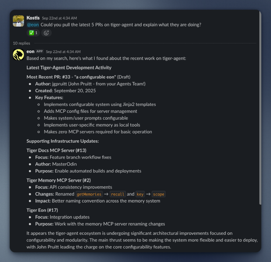
- What did we ship last week?
- What's blocking the release?
- Summarize the latest GitHub pull requests.
Eon responds instantly, pulling from the tools you already use. No new UI, no new workflow, just answers in Slack.
- Unlocks hidden value: your data in Slack, GitHub, and Linear already contains the insights you need. Eon makes them accessible.
- Enables faster decisions: no need to search or ask around, you get answers in seconds.
- Is easy to use: Eon runs a Tiger Agent and MCP servers statelessly in lightweight Docker containers.
- Integrates seamlessly with Tiger Cloud: Eon uses a Tiger Cloud service so you securely and reliably store your company data. Prefer to self-host? Use a [Postgres instance with TimescaleDB][install-self-hosted].
Tiger Eon's real-time ingestion system connects to Slack and captures everything: every message, reaction, edit, and channel update. It can also process historical Slack exports. Eon had instant access to years of institutional knowledge from the very beginning.
All of this data is stored in your Tiger Cloud service as time-series data: conversations are events unfolding over time, and Tiger Cloud is purpose-built for precisely this. Your data is optimized by:
- Automatically partitioning the data into 7-day chunks for efficient queries
- Compressing the data after 45 days to save space
- Segmenting by channel for faster retrieval
When someone asks Eon a question, it uses simple SQL to instantly retrieve the full thread context, related conversations, and historical decisions. No rate limits. No API quotas. Just direct access to your data.
This page shows you how to install and run Eon.
To follow the procedure on this page you need to:
- Create a [Tiger Data account][create-account].
This procedure also works for [self-hosted TimescaleDB][enable-timescaledb].
- [Install Docker][install-docker] on your developer device
- Install [Tiger CLI][tiger-cli]
- Have rights to create an [Anthropic API key][claude-api-key]
- Optionally:
- Have rights to create a [GitHub token][github-token]
- Have rights to create a [Logfire token][logfire-token]
- Have rights to create a [Linear token][linear-token]
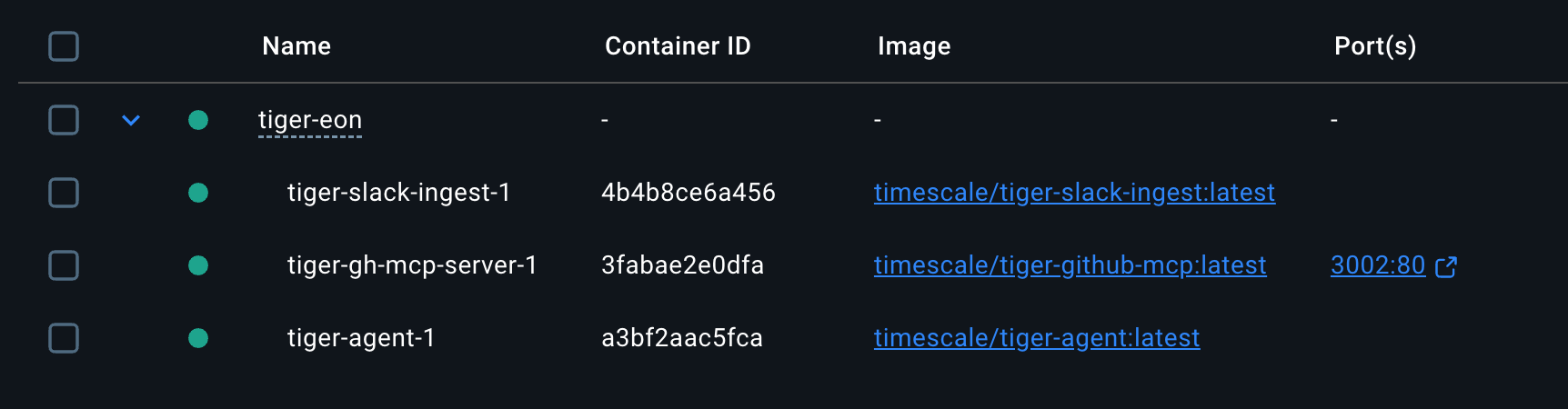
Tiger Eon is a production-ready repository running [Tiger CLI][tiger-cli] and [Tiger Agents for Work][tiger-agents] that creates and runs the following components for you:
- An ingest Slack app that consumes all messages and reactions from public channels in your Slack workspace
- A [Tiger Agent][tiger-agents] that analyzes your company data for you
- A Tiger Cloud service instance that stores data from the Slack apps
- MCP servers that connect data sources to Eon
- A listener Slack app that passes questions to the Tiger Agent when you @tag it in a public channel, and returns the AI analysis on your data
All local components are run in lightweight Docker containers via Docker Compose.
This section shows you how to run the Eon setup to configure Eon to connect to your Slack app, and give it access to your data and analytics stored in Tiger Cloud.
- Install Tiger Eon to manage and run your AI-powered Slack bots
In a local folder, run the following command from the terminal:
- Start the Eon setup
You see a summary of the setup procedure. Type y and press Enter.
- Create the Tiger Cloud service to use with Eon
You see Do you want to use a free tier Tiger Cloud Database? [y/N]:. Press Y to create a free
Tiger Cloud service.
Eon opens the Tiger Cloud authentication page in your browser. Click Authorize. Eon creates a
Tiger Cloud service called [tiger-eon][services-portal] and stores the credentials in your local keychain.
If you press N, the Eon setup creates and runs TimescaleDB in a local Docker container.
Create the ingest Slack app
In the terminal, name your ingest Slack app:
Eon proposes to create an ingest app called
tiger-slack-ingest, pressEnter.- Do the same for the App description.
Eon opens Your Apps in https://api.slack.com/apps/.
- Start configuring your ingest app in Slack:
In the Slack Your Apps page:
  1. Click `Create New App`, click `From an manifest`, then select a workspace.
  1. Click `Next`. Slack opens `Create app from manifest`.
Add the Slack app manifest:
- In terminal press
Enter. The setup prints the Slack app manifest to terminal and adds it to your clipboard. - In the Slack
Create app from manifestwindow, paste the manifest. - Click
Next, then clickCreate.
- In terminal press
Configure an app-level token:
In your app settings, go to
Basic Information.- Scroll to
App-Level Tokens. - Click
Generate Token and Scopes. - Add a
Token Name, then clickAdd Scopeaddconnections:write, then clickGenerate. - Copy the
xapp-*token and clickDone. - In the terminal, paste the token, then press
Enter.
- Scroll to
Configure a bot user OAuth token:
In your app settings, under
Features, clickApp Home.- Scroll down, then enable
Allow users to send Slash commands and messages from the messages tab. - In your app settings, under
Settings, clickInstall App. - Click
Install to <workspace name>, then clickAllow. - Copy the
xoxb-Bot User OAuth Token locally. - In the terminal, paste the token, then press
Enter.
- Scroll down, then enable
Create the Eon Slack app
Follow the same procedure as you did for the ingest Slack app.
- Integrate Eon with Anthropic
The Eon setup opens https://console.anthropic.com/settings/keys. Create a Claude Code key, then paste it in the terminal.
- Integrate Eon with Logfire
If you would like to integrate logfire with Eon, paste your token and press Enter. If not, press Enter.
- Integrate Eon with GitHub
The Eon setup asks if you would like to `Enable github MCP server?". For Eon to answer questions
about the activity in your Github organization`. Press `y` to integrate with GitHub.
- Integrate Eon with Linear
The Eon setup asks if you would like to Enable linear MCP server? [y/N]:. Press y to integrate with Linear.
Give Eon access to private repositories
The setup asks if you would like to include access to private repositories. Press
y.- Follow the GitHub token creation process.
- In the Eon setup add your organization name, then paste the GitHub token.
The setup sets up a new Tiger Cloud service for you called tiger-eon, then starts Eon in Docker.
You have created:
- The Eon ingest and chat apps in Slack
- A private MCP server connecting Eon to your data in GitHub
- A Tiger Cloud service that securely stores the data used by Eon
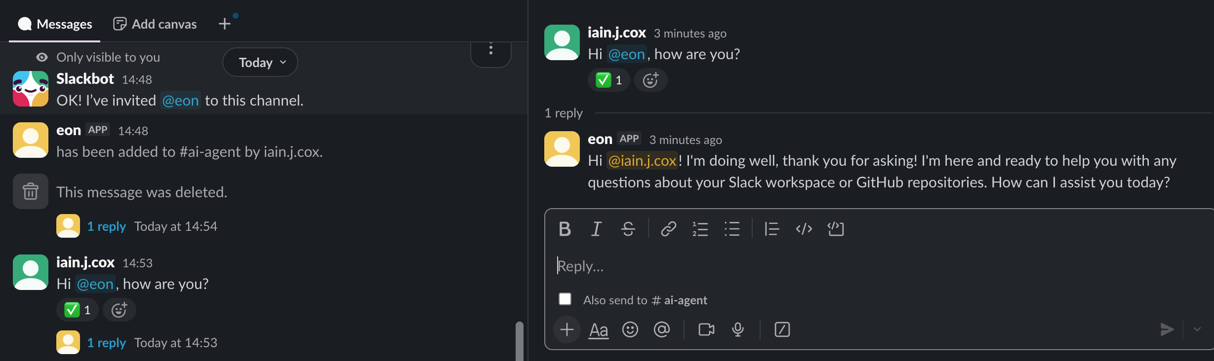
Integrate Eon in your Slack workspace
To enable your AI Assistant to analyze your data for you when you ask a question, open a public channel,
invite @eon to join, then ask a question:
===== PAGE: https://docs.tigerdata.com/ai/tiger-agents-for-work/ =====
Examples:
Example 1 (shell):
git clone git@github.com:timescale/tiger-eon.git
Example 2 (shell):
cd tiger-eon
   ./setup-tiger-eon.sh
Create candlestick aggregates
URL: llms-txt#create-candlestick-aggregates
Contents:
- Create continuous aggregates for candlestick data
- 1-minute candlestick
- 1-hour candlestick
- 1-day candlestick
- Optional: add price change (delta) column in the candlestick view
- Using multiple continuous aggregates
Turning raw, real-time tick data into aggregated candlestick views is a common task for users who work with financial data. If your data is not tick data, for example if you receive it in an already aggregated form such as 1-min buckets, you can still use these functions to help you create additional aggregates of your data into larger buckets, such as 1-hour or 1-day buckets. If you want to work with pre-aggregated stock and crypto data, see the [Analyzing Intraday Stock Data][intraday-tutorial] tutorial for more examples.
TimescaleDB includes [hyperfunctions][hyperfunctions] that you can use to
store and query your financial data more
easily. Hyperfunctions are SQL functions within TimescaleDB that make it
easier to manipulate and analyze time-series data in Postgres with fewer
lines of code. There are three
hyperfunctions that are essential for calculating candlestick values:
[time_bucket()][time-bucket], [FIRST()][first], and [LAST()][last].
The time_bucket() hyperfunction helps you aggregate records into buckets of
arbitrary time intervals based on the timestamp value. FIRST() and LAST()
help you calculate the opening and closing prices. To calculate
highest and lowest prices, you can use the standard Postgres aggregate
functions MIN and MAX.
In this first SQL example, use the hyperfunctions to query the tick data, and turn it into 1-min candlestick values in the candlestick format:
Hyperfunctions in this query:
time_bucket('1 min', time): creates 1-minute bucketsFIRST(price, time): selects the firstpricevalue in the bucket, ordered bytime, which is the opening price of the candlestick.LAST(price, time)selects the lastpricevalue in the bucket, ordered bytime, which is the closing price of the candlestick
Besides the hyperfunctions, you can see other common SQL aggregate functions
like MIN and MAX, which calculate the lowest and highest prices in the
candlestick.
This tutorial uses the LAST() hyperfunction to calculate the volume within a bucket, because
the sample tick data already provides an incremental day_volume field which
contains the total volume for the given day with each trade. Depending on the
raw data you receive and whether you want to calculate volume in terms of
trade count or the total value of the trades, you might need to use
COUNT(*), SUM(price), or subtraction between the last and first values
in the bucket to get the correct result.
Create continuous aggregates for candlestick data
In TimescaleDB, the most efficient way to create candlestick views is to use [continuous aggregates][caggs]. Continuous aggregates are very similar to Postgres materialized views but with three major advantages.
First, materialized views recreate all of the data any time the view is refreshed, which causes history to be lost. Continuous aggregates only refresh the buckets of aggregated data where the source, raw data has been changed or added.
Second, continuous aggregates can be automatically refreshed using built-in, user-configured policies. No special triggers or stored procedures are needed to refresh the data over time.
Finally, continuous aggregates are real-time by default. Any new raw tick data that is inserted between refreshes is automatically appended to the materialized data. This keeps your candlestick data up-to-date without having to write special SQL to UNION data from multiple views and tables.
Continuous aggregates are often used to power dashboards and other user-facing applications, like price charts, where query performance and timeliness of your data matter.
Let's see how to create different candlestick time buckets - 1 minute, 1 hour, and 1 day - using continuous aggregates with different refresh policies.
1-minute candlestick
To create a continuous aggregate of 1-minute candlestick data, use the same query that you previously used to get the 1-minute OHLCV values. But this time, put the query in a continuous aggregate definition:
When you run this query, TimescaleDB queries 1-minute aggregate values of all your tick data, creating the continuous aggregate and materializing the results. But your candlestick data has only been materialized up to the last data point. If you want the continuous aggregate to stay up to date as new data comes in over time, you also need to add a continuous aggregate refresh policy. For example, to refresh the continuous aggregate every two minutes:
The continuous aggregate refreshes every hour, so every hour new candlesticks are materialized, if there's new raw tick data in the hypertable.
When this job runs, it only refreshes the time period between start_offset
and end_offset, and ignores modifications outside of this window.
In most cases, set end_offset to be the same or bigger as the
time bucket in the continuous aggregate definition. This makes sure that only full
buckets get materialized during the refresh process.
1-hour candlestick
To create a 1-hour candlestick view, follow the same process as in the previous step, except this time set the time bucket value to be one hour in the continuous aggregate definition:
Add a refresh policy to refresh the continuous aggregate every hour:
Notice how this example uses a different refresh policy with different parameter values to accommodate the 1-hour time bucket in the continuous aggregate definition. The continuous aggregate will refresh every hour, so every hour there will be new candlestick data materialized, if there's new raw tick data in the hypertable.
1-day candlestick
Create the final view in this tutorial for 1-day candlesticks using the same process as above, using a 1-day time bucket size:
Add a refresh policy to refresh the continuous aggregate once a day:
The refresh job runs every day, and materializes two days' worth of candlesticks.
Optional: add price change (delta) column in the candlestick view
As an optional step, you can add an additional column in the continuous aggregate to calculate the price difference between the opening and closing price within the bucket.
In general, you can calculate the price difference with the formula:
Calculate delta in SQL:
The full continuous aggregate definition for a 1-day candlestick with a price-change column:
Using multiple continuous aggregates
You cannot currently create a continuous aggregate on top of another continuous aggregate. However, this is not necessary in most cases. You can get a similar result and performance by creating multiple continuous aggregates for the same hypertable. Due to the efficient materialization mechanism of continuous aggregates, both refresh and query performance should work well.
===== PAGE: https://docs.tigerdata.com/tutorials/OLD-financial-candlestick-tick-data/query-candlestick-views/ =====
Examples:
Example 1 (sql):
-- Create the candlestick format
SELECT
    time_bucket('1 min', time) AS bucket,
    symbol,
    FIRST(price, time) AS "open",
    MAX(price) AS high,
    MIN(price) AS low,
    LAST(price, time) AS "close",
    LAST(day_volume, time) AS day_volume
FROM crypto_ticks
GROUP BY bucket, symbol
Example 2 (sql):
/* 1-min candlestick view*/
CREATE MATERIALIZED VIEW one_min_candle
WITH (timescaledb.continuous) AS
    SELECT
        time_bucket('1 min', time) AS bucket,
        symbol,
        FIRST(price, time) AS "open",
        MAX(price) AS high,
        MIN(price) AS low,
        LAST(price, time) AS "close",
        LAST(day_volume, time) AS day_volume
    FROM crypto_ticks
    GROUP BY bucket, symbol
Example 3 (sql):
/* Refresh the continuous aggregate every two minutes */
SELECT add_continuous_aggregate_policy('one_min_candle',
    start_offset => INTERVAL '2 hour',
    end_offset => INTERVAL '10 sec',
    schedule_interval => INTERVAL '2 min');
Example 4 (sql):
/* 1-hour candlestick view */
CREATE MATERIALIZED VIEW one_hour_candle
WITH (timescaledb.continuous) AS
    SELECT
        time_bucket('1 hour', time) AS bucket,
        symbol,
        FIRST(price, time) AS "open",
        MAX(price) AS high,
        MIN(price) AS low,
        LAST(price, time) AS "close",
        LAST(day_volume, time) AS day_volume
    FROM crypto_ticks
    GROUP BY bucket, symbol